Lecture 15: Anomaly Detection

Anomaly Detection - Problem Motivation

Anomaly detection is a widely used application of machine learning. Although it can be viewed primarily as a solution to an unsupervised learning problem, it also incorporates key aspects of supervised learning.

What is Anomaly Detection?

To understand anomaly detection, consider an aircraft engine manufacturer performing quality assurance (QA) as engines roll off the assembly line:

• Feature Measurement: For each engine, measure specific features such as heat generated ($x_1$) and vibration intensity ($x_2$).
• Dataset: This yields a dataset of unlabeled features $\{x^{(1)}, x^{(2)}, \dots, x^{(m)}\}$ representing $m$ tested engines.

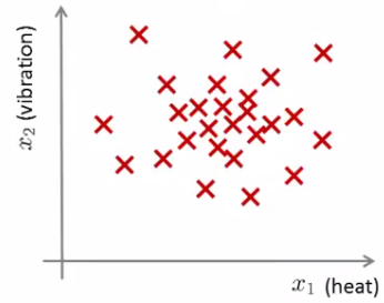
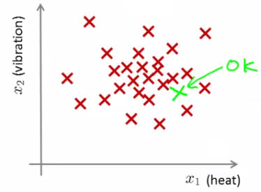
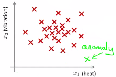
When a new engine ($x_{\text{test}}$) is produced on the next day, an anomaly detection algorithm is applied to determine if it is anomalous compared to previously manufactured engines.

• If $x_{\text{test}}$ falls within the dense region of previous data, it is classified as normal (OK).

• If $x_{\text{test}}$ falls far outside the main cluster, it is flagged as anomalous.

Formal Model Formulation

Given a dataset of normal examples $\{x^{(1)}, x^{(2)}, \dots, x^{(m)}\}$ (in practice, it is acceptable if a tiny fraction of anomalous data is present in the training set):

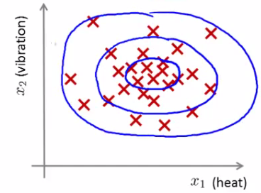
1. Density Estimation: Build a probabilistic model $p(x)$ representing the probability density that a given example $x$ is normal.
2. Decision Rule: For a new test example $x_{\text{test}}$:
   • If $p(x_{\text{test}}) < \epsilon \implies \text{Flag as anomaly}$
   • If $p(x_{\text{test}}) \ge \epsilon \implies \text{OK (Normal)}$

Here, $\epsilon$ represents a chosen threshold probability value determining how strict the system is in flagging anomalies.

---

Applications of Anomaly Detection

Fraud Detection

• Features: User behavior parameters such as online session duration, login location, transaction frequency, and spending patterns.
• Method: Build a model $p(x)$ of normal user behavior.
• Action: Identify unusual behavior patterns by passing new session data through $p(x)$. Flag suspicious accounts or automatically block fraudulent card transactions.

Manufacturing

• Quality assurance checks for manufactured components (e.g., aircraft engines, semiconductor microchips).

Data Center Computer Monitoring

• System Features: Monitor $m$ computers in a server cluster:
  • $x_1 =$ Memory usage
  • $x_2 =$ Disk accesses per second
  • $x_3 =$ CPU load
• Engineered Features: Define composite features such as $x_4 = \frac{\text{CPU load}}{\text{network traffic}}$.
• Action: Detect anomalous machines that may be failing or behaving erratically before a catastrophic cluster failure occurs.

---

Gaussian (Normal) Distribution

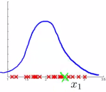
Anomaly detection heavily relies on the Gaussian (Normal) distribution.

Properties of 1D Gaussian

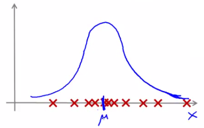
For a real-valued random variable $x \in \mathbb{R}$, if $x$ follows a Gaussian distribution with mean $\mu$ and variance $\sigma^2$ (standard deviation $\sigma$), we write:

$$x \sim \mathcal{N}(\mu, \sigma^2)$$

The probability density function is defined as:

$$p(x; \mu, \sigma^2) = \frac{1}{\sqrt{2\pi}\sigma} \exp\left( -\frac{(x - \mu)^2}{2\sigma^2} \right)$$

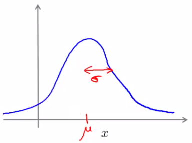
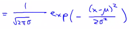
Impact of Parameters $\mu$ and $\sigma^2$

• The total area under the probability density curve always equals $1$.
• The mean $\mu$ specifies the center peak of the distribution.
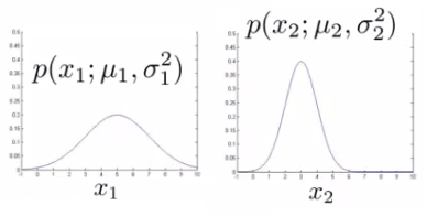
• The standard deviation $\sigma$ specifies the spread/width of the curve. Smaller $\sigma$ creates a tall, narrow peak, while larger $\sigma$ creates a wider, flatter curve.

---

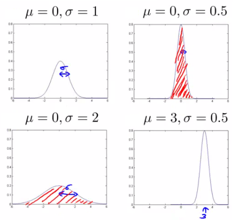
Parameter Estimation Problem

Given an unlabeled dataset of $m$ real-valued scalar examples $\{x^{(1)}, x^{(2)}, \dots, x^{(m)}\}$:

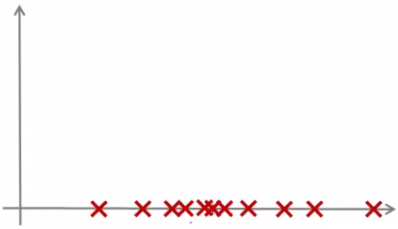
If we suspect these examples were generated from a Gaussian distribution, we can estimate the parameters $\mu$ and $\sigma^2$:

Maximum Likelihood Estimation Formulas

$$\mu = \frac{1}{m} \sum_{i=1}^{m} x^{(i)}$$ $$\sigma^2 = \frac{1}{m} \sum_{i=1}^{m} (x^{(i)} - \mu)^2$$

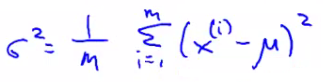
Note: In statistics, using $\frac{1}{m-1}$ instead of $\frac{1}{m}$ yields an unbiased estimate of variance. However, in machine learning, $\frac{1}{m}$ is standard; for large $m$, the numerical difference is negligible.

---

Anomaly Detection Algorithm

Model Formulation

Given an unlabeled training set of $m$ examples $\{x^{(1)}, x^{(2)}, \dots, x^{(m)}\}$ where each example $x \in \mathbb{R}^n$ is an $n$-dimensional feature vector.

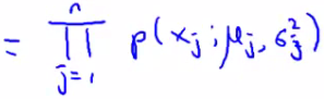
Assuming each feature $x_j$ is independently distributed according to a Gaussian distribution $x_j \sim \mathcal{N}(\mu_j, \sigma_j^2)$, the joint probability $p(x)$ is modeled as the product of individual Gaussian densities:

$$p(x) = p(x_1; \mu_1, \sigma_1^2) \cdot p(x_2; \mu_2, \sigma_2^2) \cdot \dots \cdot p(x_n; \mu_n, \sigma_n^2) = \prod_{j=1}^{n} p(x_j; \mu_j, \sigma_j^2)$$

Algorithm Steps

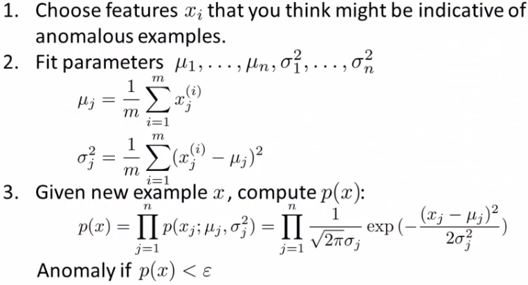
1. Feature Selection: Choose features $x_j$ indicative of general properties of the system.
2. Fit Parameters: Calculate $\mu_j$ and $\sigma_j^2$ for each feature $j = 1, \dots, n$: $$\mu_j = \frac{1}{m} \sum_{i=1}^{m} x_j^{(i)}$$ $$\sigma_j^2 = \frac{1}{m} \sum_{i=1}^{m} (x_j^{(i)} - \mu_j)^2$$
3. Evaluate Test Point: For a new test example $x_{\text{test}}$, compute $p(x_{\text{test}})$: $$p(x_{\text{test}}) = \prod_{j=1}^{n} p(x_{j,\text{test}}; \mu_j, \sigma_j^2)$$
4. Flag Anomaly: If $p(x_{\text{test}}) < \epsilon$, flag the example as an anomaly.

2D Example Walkthrough

Consider a 2D dataset with features $x_1$ and $x_2$:

• $x_1$: Mean $\mu_1 \approx 5$, standard deviation $\sigma_1 \approx 2$
• $x_2$: Mean $\mu_2 \approx 3$, standard deviation $\sigma_2 \approx 1$

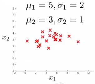
Plotting the individual feature distributions:

Multiplying the probabilities yields a 3D surface plot of $p(x)$:

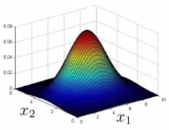
For new test examples:

• $x_{\text{test}}^{(1)}$ (normal region): $p(x_{\text{test}}^{(1)}) = 0.436 \ge \epsilon \implies \text{Normal}$
• $x_{\text{test}}^{(2)}$ (outlier region): $p(x_{\text{test}}^{(2)}) = 0.0021 < \epsilon \implies \text{Anomalous}$

---

Developing and Evaluating an Anomaly Detection System

Having a real-number evaluation metric is critical for rapidly making decisions about feature engineering, parameter choices, and model selection.

Dataset Split with Labeled Data

Even though anomaly detection is an unsupervised learning problem, having a small amount of labeled data ($y = 0$ for normal, $y = 1$ for anomalous) allows for model evaluation.

Suppose we have 10,000 normal engines ($y = 0$) and 20 anomalous engines ($y = 1$). A recommended split is:

• Training set: 6,000 normal engines ($y = 0$). Used to fit $p(x)$. (A few minor anomalies in the training set do not significantly degrade performance).
• Cross-Validation (CV) set: 2,000 normal engines ($y = 0$), 10 anomalous engines ($y = 1$).
• Test set: 2,000 normal engines ($y = 0$), 10 anomalous engines ($y = 1$).

Note: Avoid putting the same anomalous examples in both the CV and Test sets.

Evaluation Metrics

Because $y = 0$ is overwhelmingly predominant (highly skewed dataset), standard classification accuracy is a poor metric. Instead, use:

• True Positive, False Positive, False Negative, True Negative counts
• Precision and Recall
• $F_1$-score: $F_1 = 2 \cdot \frac{\text{Precision} \cdot \text{Recall}}{\text{Precision} + \text{Recall}}$

Use the cross-validation set to tune the threshold parameter $\epsilon$ by selecting the value that maximizes the $F_1$-score. Afterwards, evaluate the finalized model on the test set.

---

Anomaly Detection vs. Supervised Learning

When labeled data is available, choosing between anomaly detection and supervised learning depends on the dataset characteristics:

---

Choosing What Features to Use

Feature engineering significantly impacts anomaly detection performance.

Non-Gaussian Features

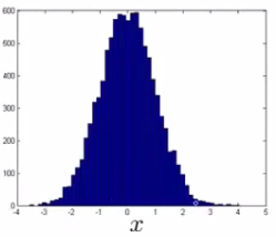
Plot a histogram of each feature (hist command in MATLAB/Octave) to verify whether it follows a Gaussian distribution.

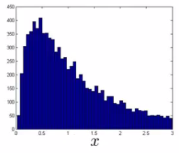
If a feature is heavily skewed, apply logarithmic or power transformations to make it more Gaussian:

• $x_1 \to \log(x_1)$
• $x_1 \to \log(x_1 + c)$
• $x_1 \to \sqrt{x_1} = x_1^{1/2}$
• $x_1 \to x_1^{1/3}$

Error Analysis for Anomaly Detection

1. Run the trained algorithm on the cross-validation set.
2. Identify false negatives (anomalous examples where $p(x) \ge \epsilon$).
3. Analyze why the algorithm assigned a high probability to the anomalous example.
4. Create a new feature that isolates the anomaly.

For example, in server monitoring, if a machine experiences unusually high CPU load while disk accesses are low, single-feature Gaussians might view both values as normal independently. Defining a new combined feature $x_4 = \frac{\text{CPU load}}{\text{network traffic}}$ or $x_5 = \frac{\text{CPU load}^2}{\text{network traffic}}$ helps highlight such anomalies.

---

Multivariate Gaussian Distribution

Motivation

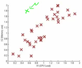
Consider an unlabeled dataset where two features ($x_1$ = CPU load, $x_2$ = memory usage) are positively correlated:

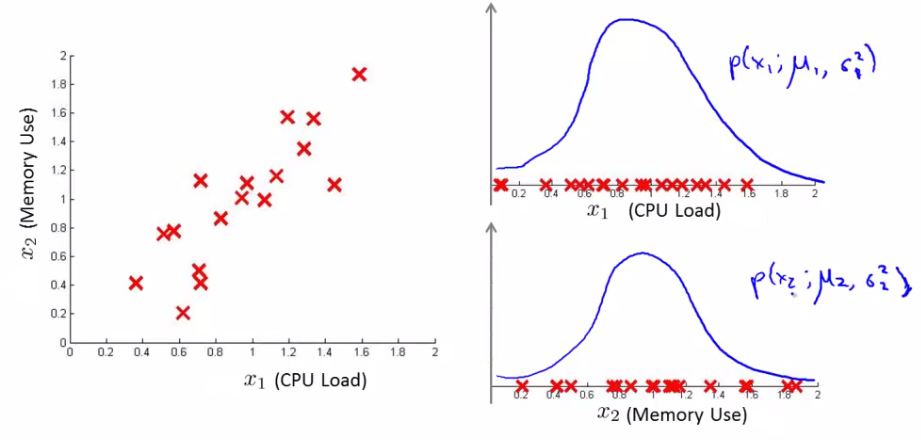
Suppose an anomalous test point occurs at $x_1 = 0.4, x_2 = 1.5$:

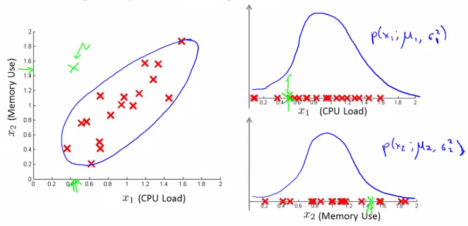
Individually, $x_1 = 0.4$ is within normal range, and $x_2 = 1.5$ is within normal range. However, their combination is highly unusual.

The original independent Gaussian model evaluates $p(x) = p(x_1)p(x_2)$, which forms axis-aligned concentric circular/elliptical contours:

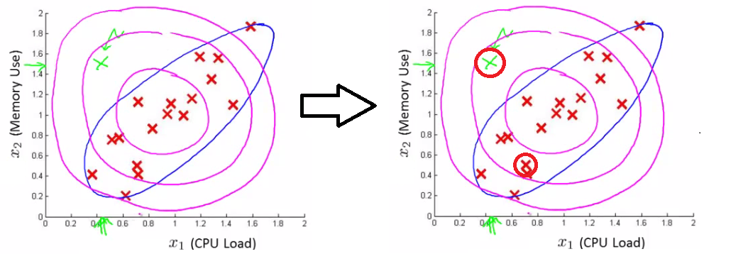
Because the concentric circles treat the green anomalous point as having the same probability density as normal points on the outer ring, the original model fails to detect the anomaly.

Mathematical Formulation

To capture feature correlations directly, use the Multivariate Gaussian Distribution.

Instead of modeling $p(x_1), p(x_2), \dots$ separately, model $p(x)$ jointly in one step using parameters:

• Mean vector $\mu \in \mathbb{R}^n$
• Covariance matrix $\Sigma \in \mathbb{R}^{n \times n}$

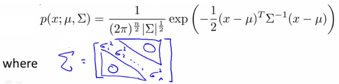
The probability density function is:

$$p(x; \mu, \Sigma) = \frac{1}{(2\pi)^{n/2} |\Sigma|^{1/2}} \exp\left( -\frac{1}{2} (x - \mu)^T \Sigma^{-1} (x - \mu) \right)$$

Where $|\Sigma|$ denotes the determinant of matrix $\Sigma$ (det(sigma) in MATLAB).

Visualizing the Effects of $\Sigma$ and $\mu$

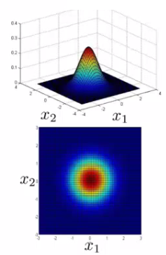
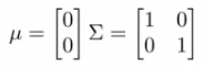
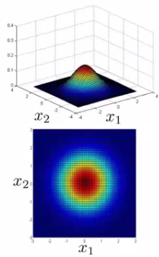
1. Standard Identity Covariance ($\Sigma = \begin{bmatrix} 1 & 0 \\ 0 & 1 \end{bmatrix}$): Symmetric bell curve centered at $\mu = \begin{bmatrix} 0 \\ 0 \end{bmatrix}$.

   

   

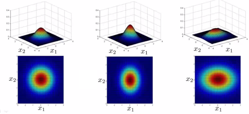
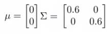
2. Shrinking Diagonal Elements ($\Sigma = \begin{bmatrix} 0.6 & 0 \\ 0 & 0.6 \end{bmatrix}$): The distribution becomes narrower and taller while maintaining axis symmetry.

   

   

3. Asymmetric Diagonal Elements: Varying individual diagonal entries alters variance along specific feature axes.

   

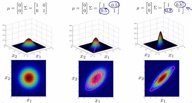
4. Off-Diagonal Elements (Correlation): Non-zero off-diagonal elements orient the elliptical contours along diagonal angles, modeling positive or negative feature correlations.

   

5. Shifting Mean $\mu$: Modifying $\mu$ translates the peak location across the feature space.

---

Anomaly Detection Algorithm with Multivariate Gaussian

Parameter Estimation

Given dataset $\{x^{(1)}, x^{(2)}, \dots, x^{(m)}\}$:

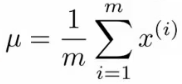
1. Mean Vector $\mu$:

   $$\mu = \frac{1}{m} \sum_{i=1}^{m} x^{(i)}$$

   

2. Covariance Matrix $\Sigma$:

   $$\Sigma = \frac{1}{m} \sum_{i=1}^{m} (x^{(i)} - \mu)(x^{(i)} - \mu)^T$$

   

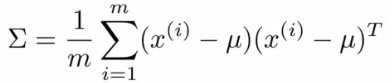
Algorithm Steps

1. Fit parameters $\mu$ and $\Sigma$ on the training set.

2. For a new test example $x_{\text{test}}$:

   

   Compute $p(x_{\text{test}})$ using the multivariate Gaussian density function:

   

3. Flag an anomaly if $p(x_{\text{test}}) < \epsilon$.

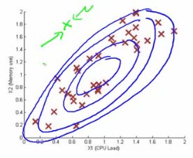
Applying Multivariate Gaussian fitting creates non-axis-aligned elliptical contours that accurately isolate the correlated anomaly:

Equivalence to Original Model

The original independent Gaussian model is a special case of the multivariate Gaussian model where the covariance matrix $\Sigma$ is constrained to be diagonal:

$$\Sigma = \begin{bmatrix} \sigma_1^2 & 0 & \dots & 0 \\ 0 & \sigma_2^2 & \dots & 0 \\ \vdots & \vdots & \ddots & \vdots \\ 0 & 0 & \dots & \sigma_n^2 \end{bmatrix}$$

---

Original Model vs. Multivariate Gaussian Model