Lecture 04: Linear Regression with Multiple Variables

Linear Regression with Multiple Features

Overview & Notation

Multivariate linear regression handles problems where we have multiple input variables (multiple features) to predict a target variable.

• Single-variable linear regression (univariate):

  • $x = \text{house size}$ (single feature)
  • $y = \text{house price}$ (target output)

• Multi-variable linear regression (multivariate):

  • Multiple features such as house size, number of bedrooms, number of floors, age of home:
    • $x_1 =$ size ($\text{sq ft}$)
    • $x_2 =$ number of bedrooms
    • $x_3 =$ number of floors
    • $x_4 =$ age of home (years)
    • $y =$ price (target output)

Notation Summary

• $n = \text{number of features}$ (e.g., $n = 4$)
• $m = \text{number of training examples}$ (number of rows in data table)
• $x^{(i)} = \text{input feature vector for the } i^{\text{th}} \text{ training example}$
  • $i$ is an index into the training set ($1 \le i \le m$)
  • $x^{(i)}$ is an $n$-dimensional feature vector
  • Example: $x^{(3)}$ represents the 4 features for the $3^{\text{rd}}$ house in the dataset
• $x_j^{(i)} = \text{value of feature } j \text{ in the } i^{\text{th}} \text{ training example}$
  • Example: $x_2^{(3)}$ represents the number of bedrooms in the $3^{\text{rd}}$ house

---

Hypothesis Representation

Previously, for a single feature, our hypothesis took the linear form:

$$h_\theta(x) = \theta_0 + \theta_1 x$$

Now, with $n$ features, our hypothesis takes the form:

$$h_\theta(x) = \theta_0 + \theta_1 x_1 + \theta_2 x_2 + \theta_3 x_3 + \dots + \theta_n x_n$$

• Example for house price prediction ($n = 4$):

$$h_\theta(x) = 80 + 0.1 x_1 + 0.01 x_2 + 3 x_3 - 2 x_4$$

Vectorized Notation

For mathematical convenience, define an extra base feature $x_0 = 1$ for every training example ($x_0^{(i)} = 1$).

This allows us to represent the feature vector $x$ and parameter vector $\theta$ as $(n+1)$-dimensional column vectors:

$$x = \begin{bmatrix} x_0 \\ x_1 \\ x_2 \\ \vdots \\ x_n \end{bmatrix} \in \mathbb{R}^{n+1}, \quad \theta = \begin{bmatrix} \theta_0 \\ \theta_1 \\ \theta_2 \\ \vdots \\ \theta_n \end{bmatrix} \in \mathbb{R}^{n+1}$$

The hypothesis can then be written as a dot product (matrix multiplication):

$$h_\theta(x) = \theta_0 x_0 + \theta_1 x_1 + \theta_2 x_2 + \dots + \theta_n x_n = \theta^T x$$

• $\theta^T$ is a $[1 \times (n+1)]$ row vector.
• $x$ is an $[(n+1) \times 1]$ column vector.
• $\theta^T x$ evaluates to a $[1 \times 1]$ scalar prediction value.

This model is known as multivariate linear regression.

---

Gradient Descent for Multiple Variables

Parameters & Cost Function

In multivariate linear regression:

• Parameters: $\theta = [\theta_0, \theta_1, \dots, \theta_n]^T \in \mathbb{R}^{n+1}$
• Cost function $J(\theta)$:

$$J(\theta) = \frac{1}{2m} \sum_{i=1}^m \left( h_\theta(x^{(i)}) - y^{(i)} \right)^2$$

Instead of viewing $J$ as a function of $n+1$ separate scalar numbers, we view $J(\theta)$ as a function of the parameter vector $\theta$.

---

Gradient Descent Algorithm

The gradient descent algorithm updates all parameters $\theta_j$ simultaneously:

$$\text{Repeat until convergence: } \left\{ \theta_j := \theta_j - \alpha \frac{\partial}{\partial \theta_j} J(\theta) \right\} \quad (\text{simultaneously update for } j = 0, \dots, n)$$

Comparing Univariate vs. Multivariate Update Rules

Single variable ($n = 1$):

$$\begin{aligned} \theta_0 &:= \theta_0 - \alpha \frac{1}{m} \sum_{i=1}^m \left( h_\theta(x^{(i)}) - y^{(i)} \right) \\ \theta_1 &:= \theta_1 - \alpha \frac{1}{m} \sum_{i=1}^m \left( h_\theta(x^{(i)}) - y^{(i)} \right) x^{(i)} \end{aligned}$$

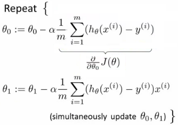
(Note that for $\theta_0$, $x_0^{(i)} = 1$ was implicitly present).

Multivariate case ($n \ge 1$):

$$\text{Repeat: } \left\{ \theta_j := \theta_j - \alpha \frac{1}{m} \sum_{i=1}^m \left( h_\theta(x^{(i)}) - y^{(i)} \right) x_j^{(i)} \right\} \quad (\text{for } j = 0, 1, \dots, n)$$

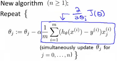
Interpretation of Update Rule

For each parameter $\theta_j$ (where $j \in \{0, \dots, n\}$):

• We update $\theta_j$ simultaneously on each iteration.
• Subtract learning rate $\alpha$ multiplied by $\frac{1}{m}$ times the sum over all $m$ examples of: (prediction error $(h_\theta(x^{(i)}) - y^{(i)})$) multiplied by (the $j^{\text{th}}$ feature value $x_j^{(i)}$ of that training example).
• The algorithms for $n=1$ and $n \ge 1$ are structurally identical.

---

Gradient Descent in Practice: Feature Scaling

Motivation

When features have significantly different scales, gradient descent can take a long time to reach the global minimum.

• Example:
  • $x_1 =$ size of house ($0 - 2000 \text{ sq ft}$)
  • $x_2 =$ number of bedrooms ($1 - 5$)
• Plotting contours of $J(\theta)$ ($\theta_1$ vs. $\theta_2$) yields extremely tall, thin ellipses due to the large difference in feature scales.

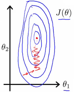
Gradient descent will oscillate back and forth across the steep walls of the narrow valley, taking a very long path and requiring many iterations to reach the minimum (pathological input).

---

Rescaling Methods

Rescaling features so they take on comparable ranges ensures contour lines are more circular, allowing gradient descent to move directly toward the minimum.

Feature Scaling (Scaling by Range/Max)

Divide each feature value by the maximum value (or range) of that feature:

$$x_1 = \frac{\text{size}}{2000}, \quad x_2 = \frac{\text{number of bedrooms}}{5}$$

• Rule of Thumb for Acceptable Feature Ranges:
  • Aim for features to be approximately in the range $-1 \le x_i \le +1$.
  • $-3 \le x_i \le +3$ is generally fine.
  • $-\frac{1}{3} \le x_i \le +\frac{1}{3}$ is okay.
  • Avoid ranges that are much larger (e.g., $-100 \text{ to } +100$) or much smaller (e.g., $-0.0001 \text{ to } +0.0001$).

Mean Normalization

Replace feature $x_i$ with $(x_i - \mu_i) / s_i$, where $\mu_i$ is the average value of feature $i$ in the training set, and $s_i$ is the range $(\text{max} - \text{min})$ or standard deviation:

$$x_i := \frac{x_i - \mu_i}{s_i}$$

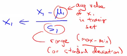
• Example for housing size ($1000 \text{ sq ft}$ average, $2000 \text{ max}$): $x_1 = \frac{\text{size} - 1000}{2000}$
• Example for bedrooms ($2 \text{ average}$, $5 \text{ max}$): $x_2 = \frac{\text{bedrooms} - 2}{5}$
• Result: Scaled features have approximately zero mean (typically $-0.5 \le x_i \le 0.5$).
• Note: Never apply feature scaling to $x_0 = 1$.

---

Gradient Descent in Practice: Learning Rate

Debugging Gradient Descent & Convergence

To ensure gradient descent is functioning properly, plot the cost function $J(\theta)$ against the number of iterations:

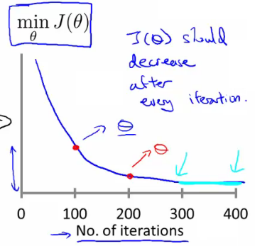
• Expected behavior: $J(\theta)$ should decrease after every single iteration.
• Convergence: When the curve flattens out, gradient descent has converged.
• Number of iterations needed: Varies widely across problems (e.g., 30 iterations, 3,000 iterations, or 3,000,000 iterations). Visualizing the $J(\theta)$ curve after 100 iterations often gives a good estimate of total iterations required.
• Automatic Convergence Test:
  • Declare convergence if $J(\theta)$ decreases by less than a small threshold $\epsilon$ (e.g., $10^{-3}$) in one iteration.
  • Setting $\epsilon$ properly can be difficult; inspecting the plot visually is usually more reliable.

---

Diagnosing Learning Rate Issues

1. Cost function increases ($J(\theta)$ rising)

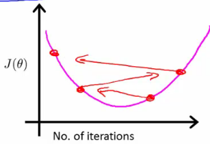
• Cause: Learning rate $\alpha$ is too large.
• Gradient descent overshoots the minimum and steps away instead of toward it.

2. Cost function oscillates (wave-like pattern)

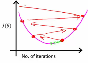
• Cause: Learning rate $\alpha$ is too large.
• Solution: Reduce the learning rate $\alpha$.

3. Summary of Learning Rate Selection

• If $\alpha$ is sufficiently small, $J(\theta)$ is guaranteed to decrease on every iteration.
• However, if $\alpha$ is too small, gradient descent will be extremely slow to converge.
• Trial range for picking $\alpha$ (3-fold steps):

$$\alpha \in \{0.001, 0.003, 0.01, 0.03, 0.1, 0.3, 1, \dots\}$$

Plot $J(\theta)$ versus iterations for each $\alpha$, and select the largest value that achieves rapid convergence without overshooting.

---

Features and Polynomial Regression

Designing New Features

You can create new features to build better prediction models.

• House price prediction example:
  • Feature $x_1 =$ frontage (width of plot along road)
  • Feature $x_2 =$ depth (depth of plot)
  • Instead of fitting $h_\theta(x) = \theta_0 + \theta_1 x_1 + \theta_2 x_2$, define a new feature:
    • $x_3 = \text{frontage} \times \text{depth} = \text{land area}$
  • Hypothesis: $h_\theta(x) = \theta_0 + \theta_1 x_3$
  • Land area $x_3$ is often a much stronger predictor of price than frontage and depth separately.

---

Polynomial Regression

When linear functions do not fit the data well, polynomial functions can provide a better model.

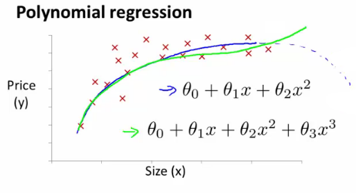
Models:

1. Quadratic model: $h_\theta(x) = \theta_0 + \theta_1 x + \theta_2 x^2$
   • Problem: Quadratic curves eventually turn back down as $x$ increases (inflection point), implying larger houses become cheaper.
2. Cubic model: $h_\theta(x) = \theta_0 + \theta_1 x + \theta_2 x^2 + \theta_3 x^3$
   • Fits data better as it continues rising.
3. Square root model: $h_\theta(x) = \theta_0 + \theta_1 x + \theta_2 \sqrt{x}$
   • Increases steadily without turning back down.

Mapping to Linear Model:

Define new features:

• $x_1 = x$
• $x_2 = x^2$
• $x_3 = x^3$

The polynomial hypothesis becomes a standard multivariate linear hypothesis:

$$h_\theta(x) = \theta_0 + \theta_1 x_1 + \theta_2 x_2 + \theta_3 x_3$$

We can apply all standard linear regression machinery directly!

Important: Feature scaling is critical for polynomial regression. If $x \in [1, 1000]$, then $x^2 \in [1, 10^6]$ and $x^3 \in [1, 10^9]$. Scale features into comparable ranges before running gradient descent.

---

Normal Equation

Overview & Intuition

For some linear regression problems, the Normal Equation provides an analytical solution to solve for $\theta$ directly in a single step without iteration.

1D Calculus Analogy

To minimize a 1D quadratic function $J(\theta) = a \theta^2 + b \theta + c$ (where $\theta \in \mathbb{R}$):

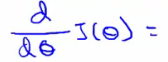
1. Take derivative $\frac{d}{d\theta} J(\theta)$
2. Set derivative to zero: $\frac{d}{d\theta} J(\theta) = 0$
3. Solve directly for $\theta$.

Multivariate Extension

For vector $\theta \in \mathbb{R}^{n+1}$:

1. Take partial derivative with respect to each parameter $\theta_j$: $\frac{\partial}{\partial \theta_j} J(\theta)$
2. Set all partial derivatives equal to zero:

$$\frac{\partial}{\partial \theta_j} J(\theta) = 0 \quad \text{for all } j = 0, \dots, n$$

3. Solve the system of equations for $\theta_0, \theta_1, \dots, \theta_n$.

---

Concrete Example

Consider a housing dataset with $m = 4$ examples and $n = 4$ features:

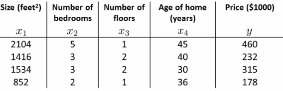
Step-by-Step Implementation:

1. Add an extra column $x_0 = 1$ for all examples.
2. Construct the Design Matrix $X$ ($[m \times (n+1)]$ matrix) containing all input features.
3. Construct the output column vector $y$ ($[m \times 1]$ vector).
4. Compute parameter vector $\theta$ using the Normal Equation:

$$\theta = (X^T X)^{-1} X^T y$$

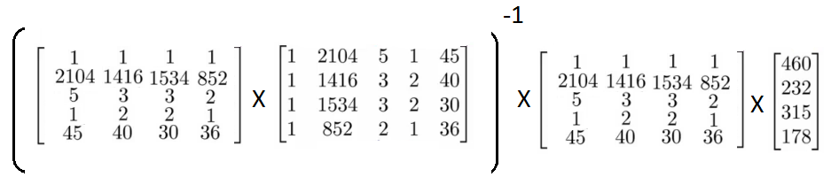
Computing this formula directly yields the vector $\theta$ that minimizes $J(\theta)$.

---

General Case

Given $m$ training examples and $n$ features:

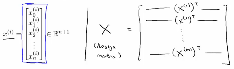
1. Design Matrix $X$ ($m \times (n+1)$): Take each example vector $x^{(i)}$ (an $(n+1)$-dimensional column vector), transpose it to a row vector $(x^{(i)})^T$, and stack as rows of $X$:

   

$$X = \begin{bmatrix} (x^{(1)})^T \\ (x^{(2)})^T \\ \vdots \\ (x^{(m)})^T \end{bmatrix} = \begin{bmatrix} x_0^{(1)} & x_1^{(1)} & \dots & x_n^{(1)} \\ x_0^{(2)} & x_1^{(2)} & \dots & x_n^{(2)} \\ \vdots & \vdots & \ddots & \vdots \\ x_0^{(m)} & x_1^{(m)} & \dots & x_n^{(m)} \end{bmatrix} \in \mathbb{R}^{m \times (n+1)}$$

2. Vector $y$ ($m \times 1$):

$$y = \begin{bmatrix} y^{(1)} \\ y^{(2)} \\ \vdots \\ y^{(m)} \end{bmatrix} \in \mathbb{R}^{m \times 1}$$

3. Normal Equation Formula:

$$\theta = (X^T X)^{-1} X^T y$$

• $(X^T X)^{-1}$ denotes the inverse of the matrix $(X^T X)$.
• In MATLAB / Octave:

  theta = pinv(X'*X) * X' * y

Feature Scaling Note: If you use the Normal Equation, feature scaling is not necessary. Gradient descent requires feature scaling to iterate efficiently, but the normal equation solves for $\theta$ exactly in one closed-form computation regardless of feature scales.

---

Gradient Descent vs. Normal Equation

---

Normal Equation and Non-Invertibility

When computing $\theta = (X^T X)^{-1} X^T y$, an edge case occurs if the matrix $(X^T X)$ is non-invertible (singular or degenerate).

• Invertibility in Practice:
  • Non-invertibility is rare in linear regression.
  • In Octave / MATLAB, using pinv(X'*X) (pseudo-inverse) calculates the correct parameters even if $(X^T X)$ is non-invertible, whereas inv(X'*X) will throw an error.

Causes of Non-Invertibility

1. Redundant Features (Linearly Dependent Features):

   • Example: $x_1 =$ size in square feet, $x_2 =$ size in square meters ($x_1 = 10.764 x_2$).
   • Solution: Remove one of the redundant features.

2. Too Many Features ($m \le n$):

   • Example: $m = 10$ training examples, $n = 100$ features (fitting 101 parameters with 10 data points).
   • Solution:
     • Delete some features.
     • Use regularization (which allows fitting models with many features and limited training data).