Lecture 13: Clustering

Unsupervised Learning - Introduction

• Talk about clustering (learning from unlabeled data)
• Unsupervised learning
  • Useful to contrast with supervised learning
• Compare and contrast:
  • Supervised learning:
    • Given a set of labels, fit a hypothesis to it
  • Unsupervised learning:
    • Try and determine structure in the data
    • Clustering algorithm groups data together based on data features
• What is clustering good for?
  • Market segmentation: Group customers into different market segments
  • Social network analysis: Facebook "smartlists"
  • Organizing computer clusters: Data centers layout and location optimization
  • Astronomical data analysis: Understanding galaxy formation

---

K-Means Algorithm

• Want an algorithm to automatically group the data into coherent clusters
• K-means is by far the most widely used clustering algorithm

Overview

• Take unlabeled data and group into two clusters:

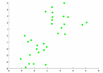
• Algorithm overview:

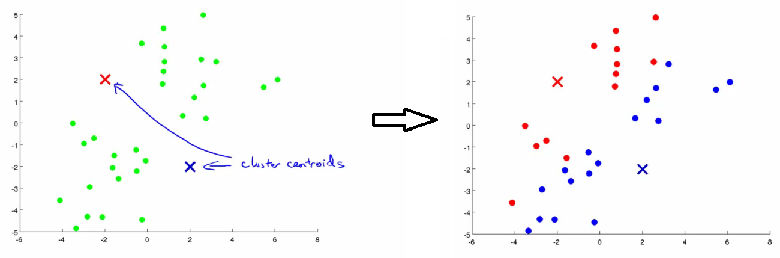
  1. Randomly allocate two points as the cluster centroids:

     • Have as many cluster centroids as clusters you want to find ($K$ cluster centroids)
     • In our example, we just have two clusters ($K = 2$)

  2. Cluster assignment step:

     • Go through each example and, depending on whether it is closer to the red or blue centroid, assign each point to one of the two clusters
     • To demonstrate this, we color each point red or blue based on proximity:

     

  3. Move centroid step:

     • Take each centroid and move it to the average (mean) of the correspondingly assigned data points:

     

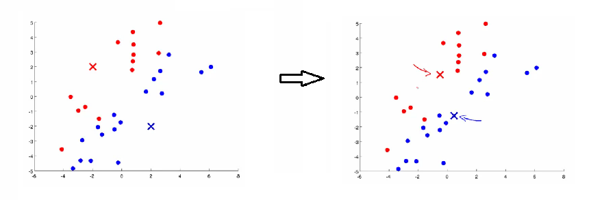
  • Repeat steps (2) and (3) until convergence.

• More formal definition:

  • Input:

    • $K$ (number of clusters in the data)
    • Training set $\{x^{(1)}, x^{(2)}, x^{(3)}, \dots, x^{(m)}\}$
    • Note: $x^{(i)} \in \mathbb{R}^n$ (by convention in clustering, drop the $x_0 = 1$ intercept term)

  • Algorithm:

  

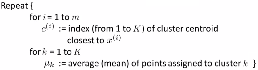
  • Randomly initialize $K$ cluster centroids $\mu_1, \mu_2, \dots, \mu_K \in \mathbb{R}^n$
  • Repeat:

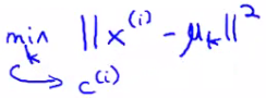
    • for i = 1 to m

      • $c^{(i)} :=$ index (from $1$ to $K$) of cluster centroid closest to $x^{(i)}$
      • i.e., take the $i$-th example, measure squared distance to each cluster centroid, assign to closest:

      

      $\min_k ||x^{(i)} - \mu_k||^2$

    • for k = 1 to K

      • $\mu_k :=$ average (mean) of points assigned to cluster $k$

K-Means for Non-Separated Clusters

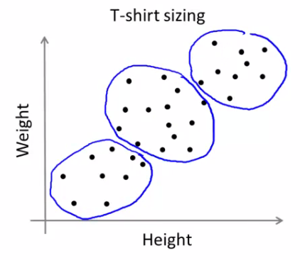
• Often K-means is applied to data that does not have well-separated, distinct clusters
• e.g., T-shirt sizing:

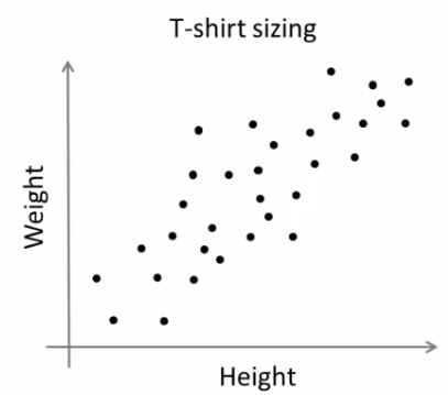
• Take height and weight features of a population
• Clusters may not look distinctly separated, but K-means can still group them into Small (S), Medium (M), and Large (L) sizes to guide product design.

---

K-Means Optimization Objective

• Most optimization algorithms in supervised learning minimize a cost function $J$. K-means also has an optimization objective function.

• Why is this useful?

  • Helps debug K-means (verify that $J$ decreases monotonically with each iteration)
  • Helps K-means avoid local optima and find better clusters

• Notation:

• $c^{(i)} =$ index of cluster $(1, 2, \dots, K)$ to which example $x^{(i)}$ is currently assigned

• $\mu_k =$ cluster centroid $k$ ($\mu_k \in \mathbb{R}^n$)

• $\mu_{c^{(i)}} =$ cluster centroid of cluster to which example $x^{(i)}$ has been assigned

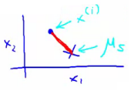
• Using this notation, we can write the optimization objective (i.e. squared distance between $x^{(i)}$ and $\mu_{c^{(i)}}$):

$J(c^{(1)}, \dots, c^{(m)}, \mu_1, \dots, \mu_K) = \frac{1}{m} \sum_{i=1}^{m} ||x^{(i)} - \mu_{c^{(i)}}||^2$

• This is just what we have been doing visually:

• The red line shows the distance between the example $x^{(i)}$ and the cluster centroid $\mu_{c^{(i)}}$ to which that example has been assigned.

• When the example is very close to the cluster centroid, this distance value is small.

• When the cluster centroid is far away from the example, the distance value is large.

• This function $J$ is sometimes called the distortion (or distortion cost function).

• So we are finding the parameter values that minimize this cost function:

$\min_{\substack{c^{(1)},\dots,c^{(m)}\\\mu_1,\dots,\mu_K}} J(c^{(1)}, \dots, c^{(m)}, \mu_1, \dots, \mu_K)$

• If we consider how the K-means algorithm operates:
  • The cluster assignment step minimizes $J(\dots)$ with respect to $c^{(1)}, c^{(2)}, \dots, c^{(m)}$ (holding $\mu_1, \dots, \mu_K$ fixed).
    • i.e., find the centroid closest to each example
    • Doesn't change the centroids themselves
  • The move centroid step minimizes $J(\dots)$ with respect to $\mu_1, \dots, \mu_K$ (holding $c^{(1)}, \dots, c^{(m)}$ fixed).
  • So, we partition the optimization process into two alternating steps:
    • First step minimizes with respect to the cluster assignment variables $c^{(i)}$
    • Second step minimizes with respect to the centroid location variables $\mu_k$
• We can use this knowledge to help debug our K-means implementation (verify that cost $J$ decreases monotonically).

---

Random Initialization

• How to initialize K-means centroids and how to avoid local optima.

• Initialization method:

  • Have the number of centroids set to less than the number of training examples ($K < m$). (If $K > m$, we cannot run K-means properly).
  • Randomly pick $K$ training examples.
  • Set $\mu_1, \dots, \mu_K$ equal to these $K$ randomly chosen training examples.

• K-means can converge to different solutions depending on the initial random setup:

  • Risk of local optima:

  

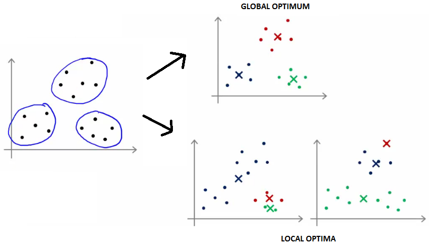
  • Local optima are valid convergence points, but they are local minima rather than global minima.

• Mitigating local optima with multiple random initializations:

  • We can perform multiple random initializations.
  • See if we arrive at the same result repeatedly — getting the same result many times strongly indicates a global optimum.

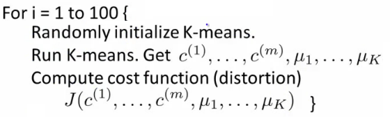
• Algorithm:

• A typical number of times to initialize K-means is between 50 and 1000.

• For i = 1 to 100 (or 50-1000):

  • Randomly initialize K-means.
  • Run K-means to convergence to obtain $c^{(1)}, \dots, c^{(m)}, \mu_1, \dots, \mu_K$.
  • Compute the distortion cost $J(c^{(1)}, \dots, c^{(m)}, \mu_1, \dots, \mu_K)$.

• Pick the clustering configuration that yielded the lowest distortion cost $J$.

• Guideline for $K$:

  • If running K-means with $K = 2 \text{ to } 10$ clusters, multiple random initializations significantly help find a better global optimum.
  • If $K > 10$, multiple random initializations are less likely to be necessary (the first random initialization usually gives a good enough clustering due to finer granularity).

---

How Do We Choose the Number of Clusters?

• Choosing $K$:
  • There is no automated, universally standard way to choose $K$.
  • Normally, visualizations or manual domain analysis are used to determine $K$.
• Why is this hard?
  • Data structure is often ambiguous (e.g. could be viewed as 2 clusters or 4 clusters — neither is inherently wrong).
  • There is not necessarily one single correct answer.

Elbow Method

• Vary $K$ and compute the cost function $J$ across a range of $K$ values.
• As $K$ increases, the minimum value of $J(\dots)$ should decrease (since higher granularity allows centroids to better fit data points).
  • Plot $K$ vs. $J(K)$.
• Look for the "elbow" point on the graph:

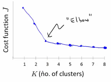
• Choose the number of clusters corresponding to the "elbow".
• If you get a clear plot, this is a reasonable method for selecting $K$.
• Limitations / Risks:
  • In practice, plots often show a smooth curve without a clear, distinct elbow.
  • Not always helpful or decisive.

Another Method for Choosing K

• Using K-means for a downstream application (e.g., market segmentation):

  • Evaluate how well different choices of $K$ serve downstream business or algorithmic needs.

• e.g., T-shirt Sizing Example:

  • Decide whether to produce 3 sizes (S, M, L) vs. 5 sizes (XS, S, M, L, XL).
  • Run K-means for $K = 3$ and $K = 5$:

  

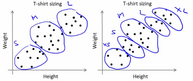
  • Choose $K$ based on trade-offs:
    • Compare the cost of manufacturing/stocking extra sizes against customer fit and satisfaction.
    • The downstream application requirements guide the selection of $K$.