Lecture 01 & 02: Introduction, Regression Analysis and Gradient Descent

Introduction to the Course

• We will learn about:
  • State-of-the-art algorithms
  • How to implement these algorithms
  • How to apply learning algorithms to real-world problems
• Applications of machine learning include:
  • Search engines
  • Photo tagging
  • Spam filters
• The AI dream of building machines as intelligent as humans:
  • Many researchers believe the most promising approach is to mimic how humans learn.
• What the course covers:
  • State-of-the-art machine learning algorithms.
  • Practical know-how: algorithms and math alone are not enough; understanding how to apply them effectively to real-world problems is essential.
• Why is Machine Learning so prevalent?
  • Grew out of Artificial Intelligence (AI).
  • Goal: Build intelligent machines.
  • Hard-wiring AI logic manually is far too difficult for complex real-world tasks.
  • The best approach is to provide a mechanism for machines to learn on their own from input data—letting the computer do the heavy lifting.

Examples of Machine Learning Applications

• Database mining:
  • Machine learning has grown rapidly due to the massive volume of data generated by modern automated systems and the web.
  • Data sources include:
    • Web data (click-stream / click-through data): Mined to understand user behavior and personalize online experiences (a major focus in Silicon Valley).
    • Medical records: Electronic medical records turned into medical knowledge and diagnostic insight.
    • Biological data: Gene sequences and microarray data giving a better understanding of the human genome.
    • Engineering data: Sensor readings, log reports, photos, and physical measurements.
• Applications that cannot be programmed by hand:
  • Autonomous helicopters
  • Handwriting recognition (e.g., automated zip code reading for postal routing)
  • Natural Language Processing (NLP)
  • Computer Vision
• Self-customizing programs:
  • Netflix, Amazon, iTunes Genius
  • Learn continuously based on individual user behavior and preferences.
• Understanding human learning and the brain:
  • Building computational systems that attempt to mimic brain function helps advance our understanding of neurobiology.

What is Machine Learning?

• Defining what machine learning is and when to use it.
• While there is no single universally accepted definition, two prominent definitions outline the field:

Arthur Samuel (1959) Definition

Machine Learning: "Field of study that gives computers the ability to learn without being explicitly programmed."

• Checkers Example: Samuel wrote a checkers-playing program and had it play 10,000 games against itself. By tracking which board positions led to wins or losses, the program learned to evaluate board positions and eventually played checkers far better than Samuel himself.

Tom Mitchell (1999) Definition

Well-posed Learning Problem: "A computer program is said to learn from experience $E$ with respect to some class of tasks $T$ and performance measure $P$, if its performance at tasks in $T$, as measured by $P$, improves with experience $E$."

• Mapping to the Checkers example:
  • Experience ($E$): Playing 10,000s of games against itself.
  • Task ($T$): Playing checkers.
  • Performance ($P$): The probability of winning against a new opponent.

Main Types of Learning Algorithms

• Supervised Learning: Teach the computer by providing correct examples, then let it apply this knowledge to new inputs.
• Unsupervised Learning: Provide unlabeled data and let the computer discover underlying structures or patterns on its own.
• Reinforcement Learning
• Recommender Systems

Course Focus: Practical advice, learning a set of tools, and how to apply them effectively to solve practical problems.

Supervised Learning - Introduction

• Supervised learning is the most common problem type in machine learning.

Example 1: Housing Price Prediction

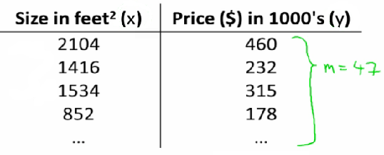
• Suppose we collect data on house prices relative to house size in square feet:

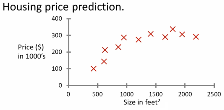
• Example Problem: "Given this data, if a friend has a 750 square foot house, how much can they expect to get for it?"
• Approaches:
  • Fit a straight line through the data $\rightarrow$ predicts approx. \150,000$.
  • Fit a second-order polynomial (quadratic curve) $\rightarrow$ predicts approx. \200,000$.
  • Later in the course, we discuss how to evaluate whether a straight line or a curved function is better suited.
• What makes this Supervised Learning?
  • We gave the algorithm a dataset containing "right answers" (actual house prices provided for each data point).
  • The algorithm learns the relationship from the training data to predict correct prices for new inputs where the output is unknown.
• This is a regression problem:
  • Predict a continuous-valued output (price). There is no discrete delineation between possible output values.

Example 2: Breast Cancer Classification

• Can we predict whether a breast tumor is malignant or benign based on tumor size?

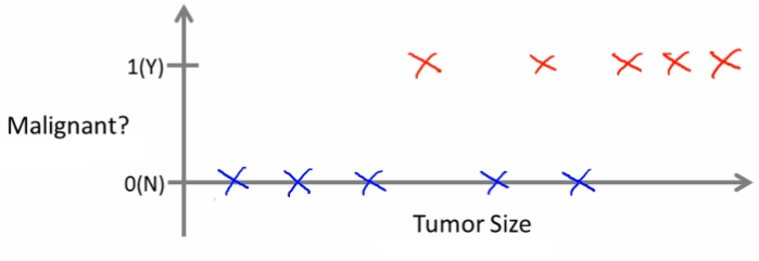
• This is an example of a classification problem:
  • Classify data into discrete categories (e.g., $0 = \text{benign}$, $1 = \text{malignant}$).
  • Output values are discrete (binary $0/1$, or multi-class such as $0 = \text{benign}$, $1 = \text{type 1}$, $2 = \text{type 2}$, $3 = \text{type 3}$).
• In classification problems, we can also plot data along a single dimension:

• When considering multiple attributes (e.g., Age and Tumor Size together):

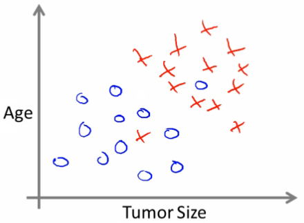
• Based on two-attribute data, we can separate classes by:
  • Drawing a straight line (linear decision boundary) between the two groups.
  • Using a more complex non-linear decision boundary.
  • Given a new patient's age and tumor size, we can classify them into one of the categories.
• Real-world problems may involve many features (e.g., clump thickness, uniformity of cell size, uniformity of cell shape).
• Advanced algorithms like Support Vector Machines (SVM) use mathematical techniques to handle an infinite number of features.

Summary of Supervised Learning

• Supervised learning provides datasets with target labels ("right answers").
• Categorized into:
  • Regression problems: Predict continuous numerical values.
  • Classification problems: Predict discrete category labels.

Unsupervised Learning - Introduction

• In unsupervised learning, we receive unlabeled data with no target output values.
• The goal is to automatically discover structure, patterns, or groupings within the data.

Clustering Algorithms

• A clustering algorithm automatically groups data points into distinct clusters.

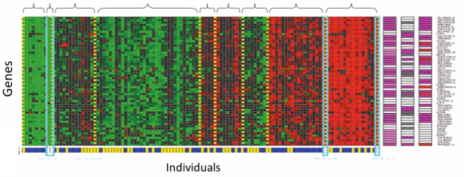
• Applications of Clustering:
  • Google News: Automatically groups thousands of daily news articles into cohesive topic clusters.
  • Genomics / Microarray data: Measures gene expression levels across individuals and clusters them into distinct genetic profiles or sub-types.
  • Computer Cluster Organization: Identifies bottlenecks and distributes compute workloads efficiently.
  • Social Network Analysis & Customer Segmentation: Groups users based on behavioral and demographic data.
  • Astronomical Data Analysis: Categorizes galaxies and cosmic phenomena.

The Cocktail Party Problem & Algorithm

• Cocktail Party Problem: Imagine a noisy room with multiple overlapping speakers. Two microphones placed at different locations record two separate mixed audio tracks.

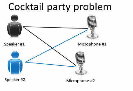
• Because the microphones are positioned at different distances from the speakers, each recording captures a slightly different mixture of the voices.
• An unsupervised learning algorithm can process these audio recordings and separate out the individual speech sources.
• Remarkably, this complex signal processing task can be implemented in Octave / MATLAB in just one line of code:

[W, s, v] = svd((repmat(sum(x .* x, 1), size(x, 1), 1) .* x) * x');

• Here, svd is the Singular Value Decomposition linear algebra routine built into Octave.
• Prototyping Note: Using high-level environments like Octave / MATLAB allows very rapid prototyping and testing of ML algorithms before porting them to languages like C++ or Python for production deployment.

Linear Regression

• Recapping the housing price prediction problem as a univariate linear regression model.

Notation

• $m$ = Number of training examples
• $x$ = Input variables / features (e.g., house size)
• $y$ = Output variable / target variable (e.g., house price)
• $(x, y)$ = Single training example
• $(x^{(i)}, y^{(i)})$ = $i$-th training example (where $i$ is an index into the training set)

• Supervised Learning Flow:
  • Pass the Training Set into the Learning Algorithm.
  • The algorithm outputs a function $h$ (called the hypothesis).
  • $h$ takes an input $x$ (e.g., size of a house) and outputs an estimated value $\hat{y}$ (the predicted price).

Representing the Hypothesis

We represent the hypothesis as a linear function:

$h_\theta(x) = \theta_0 + \theta_1 x$

(Shorthand: $h(x)$)

• This formula indicates that $y$ is modeled as a linear function of $x$.
• $\theta_0$ and $\theta_1$ are the parameters of the model:
  • $\theta_0$ represents the y-intercept (zero condition).
  • $\theta_1$ represents the slope / gradient.
• This model is called linear regression with one variable, or univariate linear regression.

Cost Function

• A cost function allows us to evaluate how well a line fits our data and choose optimal parameter values $\theta_0$ and $\theta_1$.

• We want to select parameters $(\theta_0, \theta_1)$ so that $h_\theta(x)$ is close to $y$ for all training examples $(x, y)$.
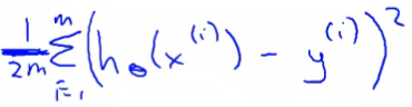
• Formally, we minimize the squared differences between the predicted values $h_\theta(x^{(i)})$ and actual values $y^{(i)}$ across all $m$ training examples:

$J(\theta_0, \theta_1) = \frac{1}{2m} \sum_{i=1}^{m} \left(h_\theta(x^{(i)}) - y^{(i)}\right)^2$

Breakdown of the Cost Function Formula:

• $\left(h_\theta(x^{(i)}) - y^{(i)}\right)$: The prediction error for example $i$.
• Squared error $\left(h_\theta(x^{(i)}) - y^{(i)}\right)^2$: Ensures all errors are positive and penalizes larger deviations more heavily.
• $\frac{1}{m}$: Computes the mean (average) squared error over the dataset.
• $\frac{1}{2}$: Included for mathematical convenience—when taking the derivative of $J(\theta_0, \theta_1)$ later, the exponent $2$ cancels out with the $\frac{1}{2}$.

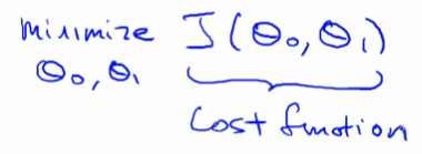
• $J(\theta_0, \theta_1)$ is known as the Squared Error Cost Function (or Mean Squared Error, MSE). It is the most standard cost function used for regression problems.

A Deeper Insight into the Cost Function

Simplified Cost Function (with $\theta_0 = 0$)

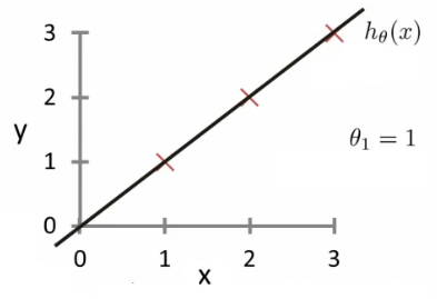
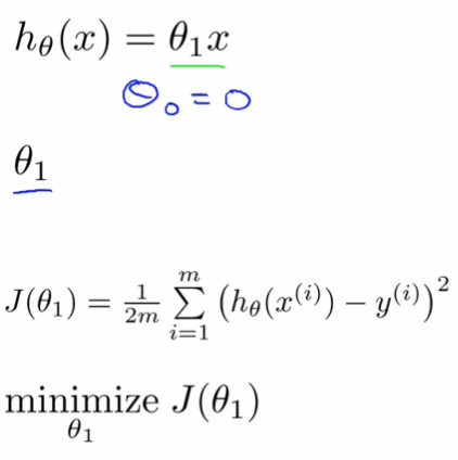
• To better visualize the cost function, let's simplify our hypothesis by setting $\theta_0 = 0$:

$h_\theta(x) = \theta_1 x$

• With $\theta_0 = 0$, the line passes through the origin $(0, 0)$.
• The cost function simplifies to:

$J(\theta_1) = \frac{1}{2m} \sum_{i=1}^{m} \left(\theta_1 x^{(i)} - y^{(i)}\right)^2$

• Key Difference to Keep in Mind:
  • $h_\theta(x)$ is a function of $x$ (for a fixed parameter value $\theta_1$). It represents the line plotted against the data points.
  • $J(\theta_1)$ is a function of the parameter $\theta_1$. It measures the total error of the hypothesis for a given value of $\theta_1$.

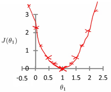
• Plotting $J(\theta_1)$ vs $\theta_1$ yields a parabola (quadratic curve).
• The optimal value of $\theta_1$ corresponds to the global minimum of $J(\theta_1)$ (where $J(\theta_1) = 0$ when $\theta_1 = 1$ in the ideal case).

Visualization with Two Parameters ($\theta_0$ and $\theta_1$)

When retaining both parameters $\theta_0$ and $\theta_1$:

• $J(\theta_0, \theta_1)$ forms a 3D surface plot shaped like a bowl:

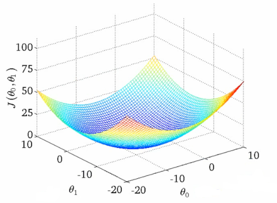
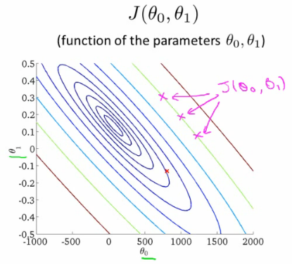
• We can also represent $J(\theta_0, \theta_1)$ using contour plots (contour figures):

• In a contour plot:
  • Each ellipse represents a constant value of $J(\theta_0, \theta_1)$.
  • The center of the concentric ellipses corresponds to the global minimum of the cost function, representing the optimal choice of parameters $(\theta_0, \theta_1)$.

Gradient Descent Algorithm

• Gradient descent is an iterative optimization algorithm used to minimize any cost function $J(\theta_0, \theta_1)$ (and more general functions $J(\theta_0, \theta_1, \dots, \theta_n)$).

How Gradient Descent Works:

1. Start with initial guesses for $\theta_0$ and $\theta_1$ (e.g., $\theta_0 = 0, \theta_1 = 0$).
2. Continuously adjust $\theta_0$ and $\theta_1$ in the direction of steepest descent to reduce $J(\theta_0, \theta_1)$.
3. Repeat until reaching a minimum.

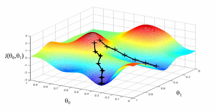
• Note on Local Minima: For general non-convex surface plots, starting at different initial points can lead gradient descent to different local minima.

Formal Definition of Gradient Descent

Repeat until convergence:

$\theta_j := \theta_j - \alpha \frac{\partial}{\partial \theta_j} J(\theta_0, \theta_1) \quad (\text{for } j = 0 \text{ and } j = 1)$

• Notation & Terms:
  • := represents assignment (overwriting the variable value).
  • $\alpha$ (alpha) is the learning rate. It controls how large a step we take downhill.
  • $\frac{\partial}{\partial \theta_j} J(\theta_0, \theta_1)$ is the partial derivative of the cost function with respect to parameter $\theta_j$.

Important Implementation Detail: Simultaneous Update

When implementing gradient descent for multiple parameters, you MUST update $\theta_0$ and $\theta_1$ simultaneously:

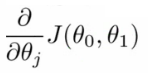
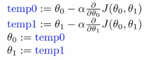
Correct Simultaneous Update:

$\text{temp0} := \theta_0 - \alpha \frac{\partial}{\partial \theta_0} J(\theta_0, \theta_1)$ $\text{temp1} := \theta_1 - \alpha \frac{\partial}{\partial \theta_1} J(\theta_0, \theta_1)$ $\theta_0 := \text{temp0}$ $\theta_1 := \text{temp1}$

Incorrect (Non-Simultaneous) Update:

$\theta_0 := \theta_0 - \alpha \frac{\partial}{\partial \theta_0} J(\theta_0, \theta_1)$ $\theta_1 := \theta_1 - \alpha \frac{\partial}{\partial \theta_1} J(\theta_0, \theta_1) \quad \text{(Error: uses the already updated } \theta_0\text{!)}$

Updating parameters sequentially rather than simultaneously changes the mathematical behavior and is NOT gradient descent.

Understanding Derivative Term and Learning Rate $\alpha$

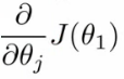
• The Derivative Term:

  • The derivative measures the slope of the tangent line at the current point.
  • If slope is positive ($\frac{d}{d\theta} J(\theta) > 0$), updating $\theta := \theta - \alpha (\text{positive})$ decreases $\theta$, moving it left toward the minimum.
  • If slope is negative ($\frac{d}{d\theta} J(\theta) < 0$), updating $\theta := \theta - \alpha (\text{negative})$ increases $\theta$, moving it right toward the minimum.

• The Learning Rate $\alpha$:

  • If $\alpha$ is too small: Gradient descent takes tiny steps and converges extremely slowly.
  • If $\alpha$ is too large: Gradient descent can overshoot the minimum, fail to converge, or even diverge.
  • As gradient descent approaches a local minimum, the derivative automatically becomes smaller, meaning gradient descent naturally takes smaller steps near the minimum even with a fixed learning rate $\alpha$.

Linear Regression with Gradient Descent

• Applying gradient descent to minimize our specific linear regression cost function $J(\theta_0, \theta_1)$:

Deriving the Partial Derivatives

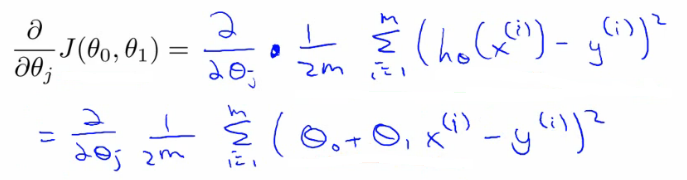
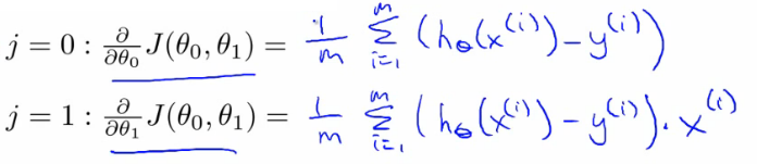
We take the partial derivative of $J(\theta_0, \theta_1)$ with respect to $\theta_0$ and $\theta_1$:

For $j = 0$: $\frac{\partial}{\partial \theta_0} J(\theta_0, \theta_1) = \frac{\partial}{\partial \theta_0} \frac{1}{2m} \sum_{i=1}^{m} \left(h_\theta(x^{(i)}) - y^{(i)}\right)^2 = \frac{1}{m} \sum_{i=1}^{m} \left(h_\theta(x^{(i)}) - y^{(i)}\right)$

For $j = 1$: $\frac{\partial}{\partial \theta_1} J(\theta_0, \theta_1) = \frac{\partial}{\partial \theta_1} \frac{1}{2m} \sum_{i=1}^{m} \left(h_\theta(x^{(i)}) - y^{(i)}\right)^2 = \frac{1}{m} \sum_{i=1}^{m} \left(h_\theta(x^{(i)}) - y^{(i)}\right) \cdot x^{(i)}$

Linear Regression Gradient Descent Algorithm

Repeat until convergence:

$\theta_0 := \theta_0 - \alpha \frac{1}{m} \sum_{i=1}^{m} \left(h_\theta(x^{(i)}) - y^{(i)}\right)$

$\theta_1 := \theta_1 - \alpha \frac{1}{m} \sum_{i=1}^{m} \left(h_\theta(x^{(i)}) - y^{(i)}\right) \cdot x^{(i)}$

(Remember: updates to $\theta_0$ and $\theta_1$ must be performed simultaneously!)

Convexity of the Cost Function

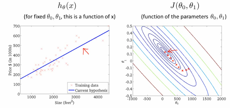
• The cost function for linear regression is a convex quadratic function ("bowl-shaped").
• Convex functions have no local minima other than the single global minimum.
• Therefore, gradient descent on linear regression will always converge to the global minimum (provided the learning rate $\alpha$ is appropriate).

"Batch" Gradient Descent

• This method is called "Batch" Gradient Descent because each step of gradient descent uses the entire batch of all training examples (summing over $i=1 \dots m$).

Alternative Optimization: The Normal Equation

• Instead of using iterative gradient descent, we can solve for optimal parameters analytically using linear algebra via the Normal Equation.
• Advantages:
  • No need to select a learning rate $\alpha$.
  • Solves directly in one step without iterations.
• Disadvantages:
  • Involves computing matrix inversion $(X^T X)^{-1}$, which becomes computationally expensive ($O(n^3)$) when feature count $n$ is very large (e.g., $n > 10,000$).
• Normal Equations are covered in detail in the multivariate linear regression section.

Extending to Multiple Features

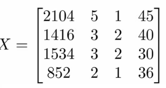
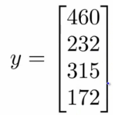
• Real-world prediction problems often involve multiple features (e.g., predicting housing price using house size, age, number of bedrooms, and number of floors):
  • Features: $x_1, x_2, x_3, x_4$

• Plotting data beyond 3 dimensions is impossible.
• Using linear algebra (matrices and vectors) provides compact mathematical notation and computationally efficient implementation (vectorization) for multi-feature regression models.