Lecture 03: Linear Algebra Review

Matrices - Overview

A matrix is a rectangular array of numbers written between square brackets.

• 2D Array: Matrices are represented as two-dimensional arrays.
• Naming: Named using capital letters (e.g., $A, B, X, Y$).
• Dimensions: The dimensions of a matrix are defined as $[\text{Rows} \times \text{Columns}]$.
  • Count starting from top-left, down to bottom-left, and across to bottom-right.
  • $\mathbb{R}^{r \times c}$ denotes a matrix with $r$ rows and $c$ columns.

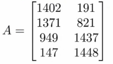
• The example matrix above is a $[4 \times 2]$ matrix.

Matrix Elements

• $A_{i,j} = \text{entry in } i^{\text{th}} \text{ row and } j^{\text{th}} \text{ column}$.

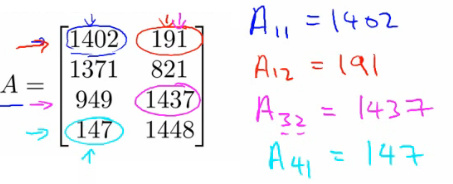
Matrices provide a powerful way to organize, index, and access large volumes of data.

---

Vectors - Overview

A vector is a matrix with $n$ rows and 1 column ($n \times 1$ matrix).

• Naming: Usually denoted by lower-case letters (e.g., $v, x, y$).
• Dimensions: Has $n$ rows and 1 column.

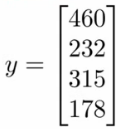
• The example above is a 4-dimensional vector, referred to as belonging to $\mathbb{R}^4$.

Vector Elements

• $v_i = i^{\text{th}} \text{ element of the vector}$.
• Indexing:
  • Vectors can be 0-indexed (common in C/C++) or 1-indexed (common in MATLAB).
  • In standard mathematics, 1-indexing is most common.
  • In machine learning implementations, 0-indexing is frequently useful.
  • Normally assume 1-indexed vectors unless explicitly specified as 0-indexed.

---

Matrix Manipulation

Addition

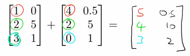
• Add corresponding elements one at a time.
• Can only add matrices of the same dimensions.
• Addition yields a new matrix of the exact same dimensions as the operands.

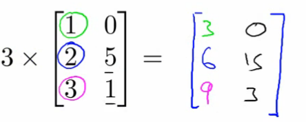
Multiplication by Scalar

• Scalar: A real number.
• Multiply every element of the matrix by the scalar.
• Generates a matrix of the same dimensions as the original matrix.

Division by Scalar

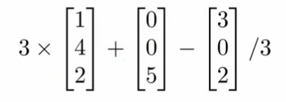
• Equivalent to multiplying the matrix by $\frac{1}{\text{scalar}}$ (e.g., multiplying by $\frac{1}{4}$).
• Each element is divided by the scalar.

Combination of Operands

• Standard order of operations applies: evaluate scalar multiplications first before additions.

Matrix-Vector Multiplication

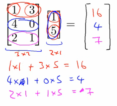
Multiplying a $[3 \times 2]$ matrix by a $[2 \times 1]$ vector yields a $[3 \times 1]$ vector.

• General Rule: Multiplying an $[a \times b]$ matrix by a $[b \times c]$ matrix/vector yields an $[a \times c]$ result.
• Procedure:
  1. Take the elements of the vector and multiply them with the corresponding elements of the matrix's first row, then sum the results to get the first element of the new vector.
  2. Repeat the step for the second row of the matrix to get the second element.
  3. Repeat for the final row to complete the new vector.

Detailed Rules

For $A \times x = y$:

• $A$ is an $m \times n$ matrix.
• $x$ is an $n \times 1$ vector.
• The inner dimensions ($n$) must match between the matrix and vector.
• The result $y$ is an $m$-dimensional vector ($m \times 1$).
• To calculate $y_i$, multiply the elements of $A$'s $i^{\text{th}}$ row by all the corresponding elements of vector $x$ and sum them up.

Vectorization Trick for Machine Learning

Suppose we have a dataset with four samples and a hypothesis function: $h_\theta(x) = -40 + 0.25x$

Instead of computing predictions individually:

1. Represent your dataset as a data matrix.
2. Put parameters ($\theta_0, \theta_1$) into a column vector.
3. Compute predictions in a single matrix-vector multiplication: $\text{Prediction} = \text{Data Matrix} \times \text{Parameters}$

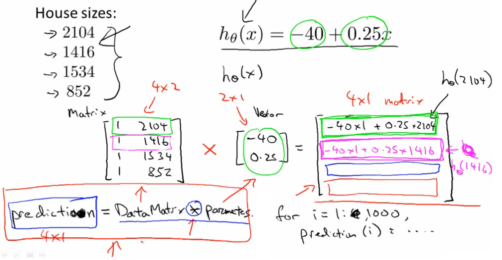
• Key Step: Add an extra column of 1s to the data matrix (representing $x_0 = 1$) so that the intercept parameter $\theta_0$ is properly calculated.
• Efficiency: This matrix formulation is computationally far more efficient than explicit for loops and produces cleaner, more concise code when using optimized linear algebra libraries.

Matrix-Matrix Multiplication

General Concept

1. Step through the second matrix one column at a time.
2. Multiply each column vector of the second matrix by the entire first matrix, generating a column vector for each step.
3. Combine (concatenate) the resulting column vectors side-by-side to form the final matrix.

Details

For $A \times B = C$:

• $A$ is $[m \times n]$.
• $B$ is $[n \times o]$.
• $C$ is $[m \times o]$. (Note: matrix-vector multiplication is just the special case where $o = 1$).
• Multiplication is only valid if the number of columns in $A$ matches the number of rows in $B$.

Summary

The $i^{\text{th}}$ column of matrix $C$ is obtained by multiplying matrix $A$ with the $i^{\text{th}}$ column of matrix $B$.

Step-by-Step Example

Given $A \times B$:

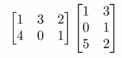
1. Multiply matrix $A$ by the 1st column vector of $B$ to get the 1st column of the result.
2. Multiply matrix $A$ by the 2nd column vector of $B$ to get the 2nd column of the result.

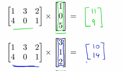
• Multiplying a $[2 \times 3]$ matrix by a $[3 \times 2]$ matrix produces a $[2 \times 2]$ matrix.

---

Implementation and Applications

Vectorizing Multiple Hypotheses

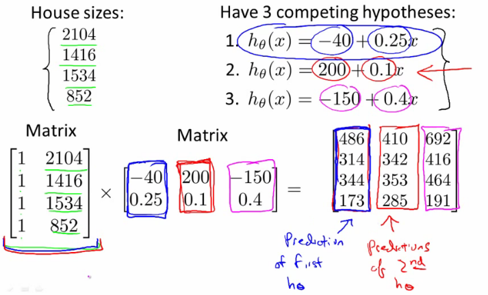
Consider a housing price dataset where we want to evaluate three competing hypotheses on the same data:

• We have 4 house sizes (samples) and want to compute predictions under 3 different hypotheses simultaneously.
• Create a $[4 \times 2]$ data matrix (house sizes with an extra column of 1s).
• Create a $[2 \times 3]$ parameter matrix where each column represents the parameters $(\theta_0, \theta_1)$ of one hypothesis.

Benefits:

• Simultaneously evaluates 3 hypotheses across 4 houses, producing all 12 predictions in a single matrix multiplication.
• Leverages optimized parallel linear algebra routines for maximum computational efficiency.

---

Matrix Multiplication Properties

While matrix multiplication is a powerful operation, it behaves differently from scalar multiplication in key ways.

Commutativity

• For scalars: $3 \times 5 = 5 \times 3$ (commutative).
• For matrices: $A \times B \neq B \times A$ in general.
• Matrix multiplication is NOT commutative.

Associativity

• For scalars: $(3 \times 5) \times 2 = 3 \times (5 \times 2) = 30$.
• For matrices: Matrix multiplication IS associative. $A \times (B \times C) = (A \times B) \times C$

Identity Matrix

• In scalar arithmetic, $1$ is the multiplicative identity ($1 \cdot z = z$).
• In matrix algebra, the Identity Matrix is denoted by $I$ (or $I_{n \times n}$).

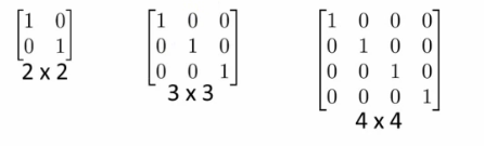
• Properties of $I$:
  • Square matrix ($n \times n$).
  • Contains $1$s along the main diagonal and $0$s everywhere else.
  • A $[1 \times 1]$ identity matrix is simply $[1]$.
• Multiplying any matrix $A$ by an appropriate identity matrix returns $A$:
  • $A \cdot I_{n \times n} = A$ (where $A$ is $[m \times n]$)
  • $I_{m \times m} \cdot A = A$ (where $A$ is $[m \times n]$)
• Exception to Commutativity: Matrix multiplication is commutative only when one of the matrices is the identity matrix ($A \cdot I = I \cdot A = A$).

---

Inverse and Transpose Operations

Matrix Inverse

Concept in Real Numbers

• The number $1$ is the multiplicative identity.
• The inverse of a number $x$ is $x^{-1} = \frac{1}{x}$, such that $x \cdot x^{-1} = 1$ (e.g., $3 \cdot 3^{-1} = 1$).
• Not all numbers have an inverse: $0$ does not have a multiplicative inverse.

Matrix Inverse Definition

• If $A$ is an $m \times m$ matrix, its inverse is $A^{-1}$ such that: $A \cdot A^{-1} = I$
• Square Matrices Only: Only square matrices ($m \times m$) can have an inverse.

Singular and Degenerate Matrices

• Matrices filled with all zeros do not have an inverse.
• Matrices that do not have an inverse are called singular or degenerate matrices (intuitively, matrices that are "too close to 0" or lack full rank).

Matrix Transpose

Concept

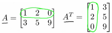
Given an $[m \times n]$ matrix $A$, the transpose $A^T$ is an $[n \times m]$ matrix formed by swapping rows and columns.

Procedure

• 1st row of $A$ becomes the 1st column of $A^T$.
• 2nd row of $A$ becomes the 2nd column of $A^T$.
• In general, for $B = A^T$: $A_{i,j} = B_{j,i}$

---

Eigenvalues and Eigenvectors

Definition and Geometric Intuition

For an $n \times n$ square matrix $A$, a non-zero vector $v \in \mathbb{R}^n$ is an eigenvector if multiplying it by $A$ yields a scaled version of itself:

$Av = \lambda v$

• $A$: An $n \times n$ transformation matrix.
• $v$: The eigenvector ($v \neq \mathbf{0}$).
• $\lambda$: The eigenvalue (a scalar scaling factor).

Geometric Meaning

Most linear transformations both rotate and stretch vectors. Eigenvectors are special invariant directions that do not rotate under the transformation—they only stretch, shrink, or flip along the same line:

• $\lambda > 1$: The vector stretches.
• $0 < \lambda < 1$: The vector shrinks.
• $\lambda < 0$: The vector flips in the opposite direction.
• $\lambda = 0$: The vector collapses to zero ($v$ lies in the null space of $A$).

Characteristic Equation

To compute eigenvalues, solve the characteristic equation: $(A - \lambda I)v = \mathbf{0} \implies \det(A - \lambda I) = 0$

---

Special Eigenvalue Properties in Theoretical Machine Learning

In probabilistic machine learning algorithms such as Gaussian Discriminant Analysis (GDA), Gaussian Mixture Models (GMM), and the Expectation-Maximization (EM) algorithm, eigenvalues play a foundational role in analyzing covariance matrices ($\Sigma$) and Hessian matrices ($H$).

1. Covariance Matrices & Positive Definiteness

Any empirical covariance matrix $\Sigma$ is symmetric ($\Sigma^T = \Sigma$) and Positive Semi-Definite (PSD) ($\Sigma \succeq 0$):

• Real Eigenvalues: All eigenvalues of a symmetric matrix are strictly real ($\lambda_i \in \mathbb{R}$).
• Non-Negative Eigenvalues: For PSD matrices, $\lambda_i \ge 0$.
• Strictly Positive Definite (PD): If $\Sigma \succ 0$, then every eigenvalue is strictly positive ($\lambda_i > 0$), guaranteeing that variance along any arbitrary projection is strictly positive.

2. Determinant as Volume ($\det(\Sigma) = \prod_{i=1}^d \lambda_i$) & The EM Singularity

The determinant of a covariance matrix is the product of its eigenvalues: $\det(\Sigma) = \prod_{i=1}^d \lambda_i$

• Gaussian Normalization: Appears in the denominator of the multivariate Gaussian probability density function: $p(x; \mu, \Sigma) = \frac{1}{(2\pi)^{d/2}|\Sigma|^{1/2}} \exp\left(-\frac{1}{2}(x-\mu)^T \Sigma^{-1}(x-\mu)\right)$
• EM Singularity Problem in GMMs: If a Gaussian component collapses onto a single data point during EM optimization, the variance along one dimension shrinks to zero ($\lambda_{\min} \to 0$). Consequently, $\det(\Sigma) \to 0$, causing $|\Sigma|^{-1/2} \to \infty$ and the likelihood objective to diverge to $+\infty$.

3. Precision Matrix ($\Omega = \Sigma^{-1}$) & Conditional Independence

If $\Sigma$ has eigenvectors $u_1, \dots, u_d$ with eigenvalues $\lambda_1, \dots, \lambda_d$, then the precision matrix $\Omega = \Sigma^{-1}$ shares the exact same eigenvectors $u_i$, but with inverted eigenvalues: $\lambda(\Sigma^{-1})_i = \frac{1}{\lambda_i}$

• Checking Conditional Independence: In a multivariate Gaussian distribution $X \sim \mathcal{N}(\mu, \Sigma)$, two variables $X_i$ and $X_j$ are conditionally independent given all other variables if and only if their corresponding off-diagonal entry in the precision matrix is zero: $X_i \perp X_j \mid X_{\text{rest}} \iff (\Sigma^{-1})_{ij} = 0$
  • Contrast this with marginal independence, which holds if and only if the covariance entry is zero: $X_i \perp X_j \iff \Sigma_{ij} = 0$.
• Mahalanobis Distance: In the quadratic form $(x-\mu)^T \Sigma^{-1} (x-\mu) = \sum_{i=1}^d \frac{1}{\lambda_i} (u_i^T (x-\mu))^2$, directions with large variance ($\lambda_i \gg 0$) receive smaller weight penalties, naturally normalizing distances across features with varying scales.

4. Spectral Decomposition & Geometric Contours of Gaussians

By the Spectral Theorem, any symmetric matrix can be decomposed into: $\Sigma = U \Lambda U^T = \sum_{i=1}^d \lambda_i u_i u_i^T$ where $U = [u_1, \dots, u_d]$ is an orthogonal matrix of eigenvectors ($U^T U = I$) and $\Lambda = \operatorname{diag}(\lambda_1, \dots, \lambda_d)$.

• Iso-Density Contours: The level curves of equal probability $\{x : (x-\mu)^T \Sigma^{-1} (x-\mu) = c^2\}$ form an ellipsoid.
• Principal Axes: The axes of the ellipsoid point along the eigenvectors $u_i$.
• Axis Radii: The half-lengths of the semi-axes are proportional to $\sqrt{\lambda_i}$ (the standard deviation along that principal direction).

5. Trace as Total Variance ($\operatorname{Tr}(\Sigma) = \sum_{i=1}^d \lambda_i$)

The trace of a square matrix equals the sum of its diagonal entries, which also equals the sum of its eigenvalues: $\operatorname{Tr}(\Sigma) = \sum_{i=1}^d \Sigma_{ii} = \sum_{i=1}^d \lambda_i$

• In feature analysis and PCA, $\operatorname{Tr}(\Sigma)$ measures the total variance across all features in the dataset.

6. Regularization (Jitter / Ridge) Shifts Eigenvalues

When applying shrinkage or diagonal jittering to stabilize covariance estimation: $\Sigma_{\text{reg}} = \Sigma + \epsilon I$

• The eigenvectors $u_i$ remain completely unchanged.
• Every eigenvalue is shifted by a constant: $\lambda_i \to \lambda_i + \epsilon$.
• Practical Benefit: Even if $\Sigma$ is singular or rank-deficient ($\lambda_{\min} = 0$), $\Sigma_{\text{reg}}$ is guaranteed to be strictly positive definite with minimum eigenvalue $\epsilon$, ensuring numerical stability when taking matrix inverses in GDA and EM.

7. Generalized Eigenvalue Problems in LDA / GDA

In Linear Discriminant Analysis (and Gaussian Discriminant Analysis with shared covariance), finding the optimal linear projection $w$ that maximizes the ratio of between-class variance $S_B$ to within-class variance $S_W$ involves maximizing the Rayleigh Quotient: $\max_w \frac{w^T S_B w}{w^T S_W w}$ Taking the gradient and setting it to zero yields the generalized eigenvalue problem: $S_B w = \lambda S_W w \implies S_W^{-1} S_B w = \lambda w$ The optimal projection direction $w$ is the eigenvector corresponding to the largest eigenvalue $\lambda_{\max}$ of $S_W^{-1} S_B$.

8. Hessians, Curvature, and Convexity in Maximum Likelihood

In optimization and Maximum Likelihood Estimation (MLE):

• The curvature of an objective function $\ell(\theta)$ is governed by its Hessian matrix $H = \nabla^2 \ell(\theta)$.
• If all eigenvalues of $H$ are strictly negative ($\lambda_i < 0 \iff H \prec 0$), the objective function is strictly concave. This guarantees that any stationary point found by gradient ascent or Newton's method is the unique global maximum (e.g., Logistic Regression, GLMs).

---

Eigenvalues in Machine Learning: Quick Reference