Lecture 07: Regularization

The Problem of Overfitting

• So far we've seen a few algorithms - work well for many applications, but can suffer from the problem of overfitting
• What is overfitting?
• What is regularization and how does it help

Overfitting with Linear Regression

• Using our house pricing example again
  • Fit a linear function to the data - not a great model
    • This is underfitting - also known as high bias
    • Bias is a historic/technical one - if we're fitting a straight line to the data we have a strong preconception that there should be a linear fit
      • In this case, this is not correct, but a straight line can't help being straight!
  • Fit a quadratic function
    • Works well
  • Fit a 4th order polynomial
    • Now curve fits through all five examples
      • Seems to do a good job fitting the training set
      • But, despite fitting the data we've provided very well, this is actually not such a good model
    • This is overfitting - also known as high variance
  • Algorithm has high variance
    • High variance - if fitting high order polynomial then the hypothesis can basically fit any data
    • Space of hypothesis is too large

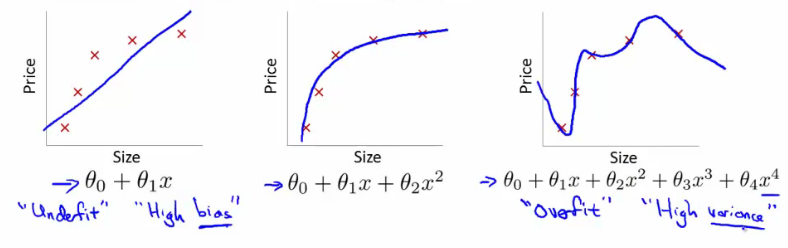
• To recap, if we have too many features then the learned hypothesis may give a cost function of exactly zero
  • But this tries too hard to fit the training set
  • Fails to provide a general solution - unable to generalize (apply to new examples)

Overfitting with Logistic Regression

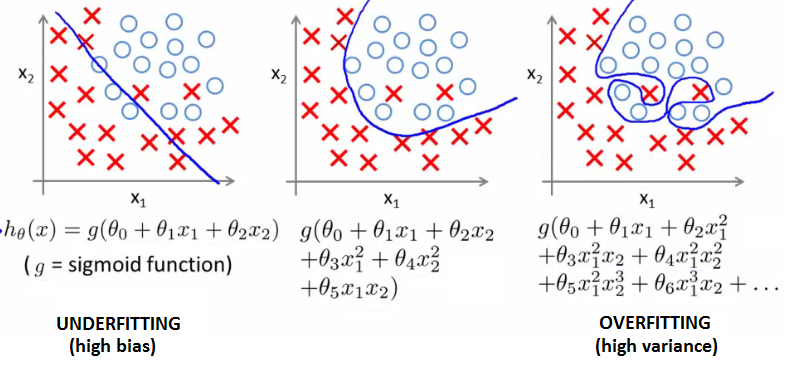
• Same thing can happen to logistic regression
  • Sigmoidal function is an underfit
  • But a high order polynomial gives an overfitting (high variance hypothesis)

Addressing Overfitting

• Later we'll look at identifying when overfitting and underfitting is occurring
• Earlier we just plotted a higher order function - saw that it looks "too curvy"
  • Plotting hypothesis is one way to decide, but doesn't always work
  • Often have lots of features - here it's not just a case of selecting a degree polynomial, but also harder to plot the data and visualize to decide what features to keep and which to drop
  • If you have lots of features and little data - overfitting can be a problem
• How do we deal with this?
  • 1. Reduce number of features
    • Manually select which features to keep
    • Model selection algorithms are discussed later (good for reducing number of features)
    • But, in reducing the number of features we lose some information
      • Ideally select those features which minimize data loss, but even so, some info is lost
  • 2. Regularization
    • Keep all features, but reduce magnitude of parameters $\theta$
    • Works well when we have a lot of features, each of which contributes a bit to predicting $y$

Cost Function Optimization for Regularization

• Penalize and make some of the $\theta$ parameters really small
  • e.g. here $\theta_3$ and $\theta_4$

• The addition in blue is a modification of our cost function to help penalize $\theta_3$ and $\theta_4$
  • So here we end up with $\theta_3$ and $\theta_4$ being close to zero (because the constants are massive)
  • So we're basically left with a quadratic function

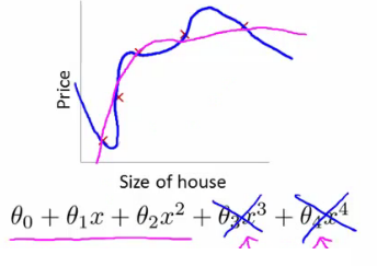
• In this example, we penalized two of the parameter values
  • More generally, regularization is as follows:
• Regularization
  • Small values for parameters corresponds to a simpler hypothesis (you effectively get rid of some of the terms)
  • A simpler hypothesis is less prone to overfitting
• Another example
  • Have 100 features $x_1, x_2, \dots, x_{100}$
  • Unlike the polynomial example, we don't know what are the high order terms
    • How do we pick the ones to shrink?
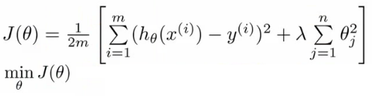
  • With regularization, take cost function and modify it to shrink all the parameters
    • Add a term at the end
      • This regularization term shrinks every parameter
      • By convention you don't penalize $\theta_0$ - minimization is from $\theta_1$ onwards

• In practice, if you include $\theta_0$ it has little impact
• $\lambda$ is the regularization parameter
  • Controls a trade off between our two goals:
    • 1. Want to fit the training set well
    • 2. Want to keep parameters small
• With our example, using the regularized objective (i.e. the cost function with the regularization term) you get a much smoother curve which fits the data and gives a much better hypothesis
  • If $\lambda$ is very large we end up penalizing ALL the parameters ($\theta_1, \theta_2$ etc.) so all the parameters end up being close to zero
    • If this happens, it's like we got rid of all the terms in the hypothesis
      • This results here is then underfitting
    • So this hypothesis is too biased because of the absence of any parameters (effectively)
• So, $\lambda$ should be chosen carefully - not too big...
  • We look at some automatic ways to select $\lambda$ later in the course

Regularized Linear Regression

• Previously, we looked at two algorithms for linear regression
  • Gradient descent
  • Normal equation
• Our linear regression with regularization is shown below

• Previously, gradient descent would repeatedly update the parameters $\theta_j$, where $j = 0,1,2 \dots n$ simultaneously
  • Shown below:

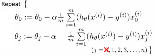
• We've got the $\theta_0$ update here shown explicitly
  • This is because for regularization we don't penalize $\theta_0$ so treat it slightly differently
• How do we regularize these two rules?
  • Take the term and add $\frac{\lambda}{m} \theta_j$
    • Sum for every $\theta$ (i.e. $j = 0$ to $n$)
  • This gives regularization for gradient descent
• We can show using calculus that the equation given below is the partial derivative of the regularized $J(\theta)$

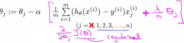
• The update for $\theta_j$:
  • $\theta_j$ gets updated to $\theta_j - \alpha \cdot [\text{a big term which also depends on } \theta_j]$
• So if you group the $\theta_j$ terms together:

• The term:

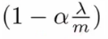
• Is going to be a number less than 1 usually
  • Usually learning rate is small and $m$ is large
    • So this typically evaluates to $(1 - \text{a small number})$
    • So the term is often around 0.99 to 0.95
• This in effect means $\theta_j$ gets multiplied by 0.99
  • Means the squared norm of $\theta_j$ a little smaller
  • The second term is exactly the same as the original gradient descent

Regularization with the Normal Equation

• Normal equation is the other linear regression model
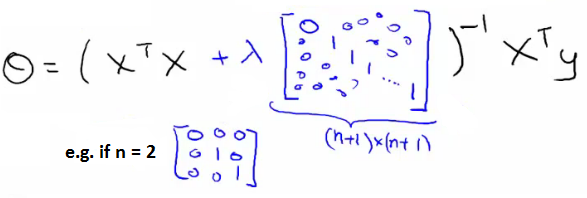
  • Minimize the $J(\theta)$ using the normal equation
  • To use regularization we add a term ($+ \lambda [n+1 \times n+1]$) to the equation
    • $[n+1 \times n+1]$ is the $n+1$ identity matrix

Regularization for Logistic Regression

• We saw earlier that logistic regression can be prone to overfitting with lots of features
• Logistic regression cost function is as follows:

• To modify it we have to add an extra term:

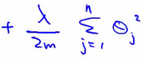
• This has the effect of penalizing the parameters $\theta_1, \theta_2$ up to $\theta_n$
  • Means, like with linear regression, we can get what appears to be a better fitting lower order hypothesis
• How do we implement this?
  • Original logistic regression with gradient descent function was as follows:

• Again, to modify the algorithm we simply need to modify the update rule for $\theta_1$, onwards
  • Looks cosmetically the same as linear regression, except obviously the hypothesis is very different

Advanced Optimization of Regularized Linear Regression

• As before, define a costFunction which takes a $\theta$ parameter and gives jVal and gradient back

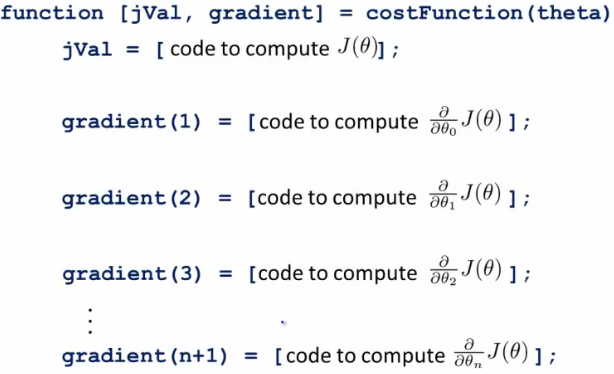
• use fminunc
  • Pass it an @costfunction argument
  • Minimizes in an optimized manner using the cost function
• jVal
  • Need code to compute $J(\theta)$
    • Need to include regularization term
• Gradient
  • Needs to be the partial derivative of $J(\theta)$ with respect to $\theta_i$
  • Adding the appropriate term here is also necessary

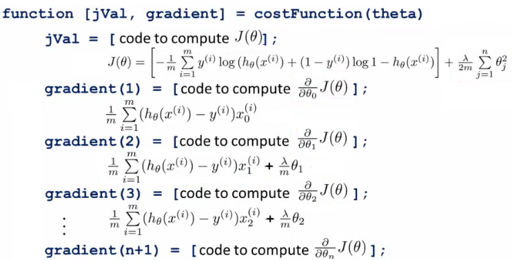
• Ensure summation doesn't extend to the lambda term!
  • It doesn't, but, you know, don't be daft!