Lecture 09: Neural Networks - Learning

Neural Network Cost Function

Neural Networks (NNs) are one of the most powerful learning algorithms. They allow fitting complex non-linear hypothesis functions given a training set. Let's first examine the setup and cost function for neural networks.

Setup and Notation

We focus on the application of NNs to classification problems. Here is the general setup:

• Training set: $\{(x^{(1)}, y^{(1)}), (x^{(2)}, y^{(2)}), (x^{(3)}, y^{(3)}), \dots, (x^{(m)}, y^{(m)})\}$
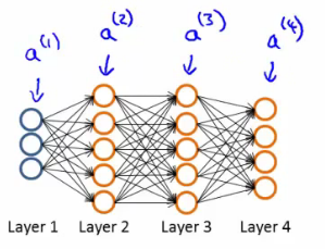
• $L$ = total number of layers in the network (e.g., $L = 4$ in the diagram below)
• $s_l$ = number of units (not counting the bias unit) in layer $l$

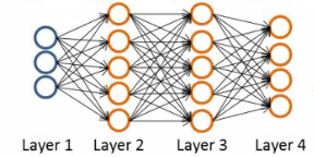
In the example network shown above:

• $L = 4$ (4 layers)
• $s_1 = 3$ (3 input features, excluding bias $x_0$)
• $s_2 = 5$ (5 hidden units in layer 2)
• $s_3 = 5$ (5 hidden units in layer 3)
• $s_4 = 4$ (4 output units in layer 4)

Types of Classification Problems

We distinguish two types of classification problems in neural networks:

• Binary classification:

  • Single output ($y \in \{0, 1\}$)
  • Output node is a scalar real number
  • $K = 1$ output unit (where $K$ denotes the number of units in the output layer)
  • $s_L = 1$

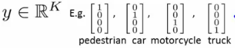
• Multi-class classification:

  • $K$ distinct classification categories ($K \ge 3$; if $K = 2$, it defaults to binary classification)
  • Output $y$ is a $K$-dimensional vector of real numbers (one-hot encoded vector representing each class)
  • $s_L = K$

Cost Function for Neural Networks

Recall that the regularized logistic regression cost function for binary classification is:

For neural networks, the cost function is a generalization of this equation. Instead of a single scalar output, the hypothesis $h_\Theta(x)$ outputs a $K$-dimensional vector:

Here:

• $h_\Theta(x) \in \mathbb{R}^K$, so $(h_\Theta(x))_k$ refers to the $k$-th element of the output vector.
• The summation $\sum_{k=1}^K$ accumulates the logistic regression loss over all $K$ output units.

Understanding the Cost Function

The neural network cost function consists of two primary components:

1. First Half (Unregularized Cost):

This term computes the average cross-entropy loss over all $m$ training examples and across all $K$ output units.

2. Second Half (Regularization / Weight Decay):

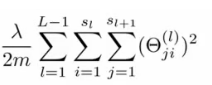
This is a triple nested summation that sums the square of every parameter weight in the network. Notice that:

• We do not regularize the bias terms ($\Theta_{j0}^{(l)}$), hence the index $i$ starts from 1. (Even if bias terms were regularized, it wouldn't make much difference, but omitting them is standard).
• This term is often called the weight decay term.
• As before, $\lambda$ balances fitting the training data versus keeping weight parameters small to prevent overfitting.

Now that we have defined the cost function $J(\Theta)$, how do we minimize it?

Overview of Training & Backpropagation

The backpropagation algorithm is one of the more involved concepts in machine learning, so let's first outline the high-level roadmap of what we are doing.

Forward Propagation vs. Backpropagation

• Forward Propagation: Takes the neural network parameters $\Theta$ and an input vector $x$, feeding it forward through each layer to compute activations up to the output hypothesis $h_\Theta(x)$ (which can be a scalar or a $K$-dimensional vector).
• Backpropagation:
  1. Takes the network's output hypothesis $h_\Theta(x)$ and compares it against the true label $y$ to compute the error of the output layer.
  2. Back-calculates the error associated with each unit in preceding hidden layers (from layer $L-1$ down to layer 2).
  3. Uses these error terms to compute the partial derivatives of the cost function $\frac{\partial}{\partial \Theta_{ij}^{(l)}} J(\Theta)$.
  4. Feeds these partial derivatives into gradient descent (or advanced optimization algorithms like BFGS, L-BFGS, conjugate gradient) to minimize $J(\Theta)$ and iteratively update $\Theta$.

Key Matrices to Keep in Mind

• For each layer $l$, there is a parameter matrix $\Theta^{(l)}$ mapping from layer $l$ to layer $l+1$. The size of $\Theta^{(l)}$ is $s_{l+1} \times (s_l + 1)$.
• There is an error matrix $\Delta^{(l)}$ associated with each layer $l$, which serves as an accumulator for computing partial derivatives across all $m$ training examples.

Backpropagation Algorithm

The backpropagation algorithm allows us to efficiently calculate the partial derivatives $\frac{\partial}{\partial \Theta_{ij}^{(l)}} J(\Theta)$ so we can minimize $J(\Theta)$.

Given the cost function $J(\Theta)$, our goal is to find parameters $\Theta$ to minimize $J(\Theta)$:

To use optimization algorithms (such as gradient descent or advanced optimizers), we need code that computes two things:

1. $J(\Theta)$: The cost value for a given set of parameters $\Theta$.
2. Partial derivative terms: $\frac{\partial}{\partial \Theta_{ij}^{(l)}} J(\Theta)$ for every parameter $\Theta_{ij}^{(l)} \in \mathbb{R}$.

Recall the index notation for $\Theta_{ij}^{(l)}$:

• $l$: origin layer (layer mapping from)
• $j$: origin node in layer $l$ (node mapping from)
• $i$: destination node in layer $l+1$ (node mapping to)

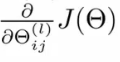
Each partial derivative term $\frac{\partial}{\partial \Theta_{ij}^{(l)}} J(\Theta)$ is a single real number.

Vectorized Forward Propagation (Single Training Example)

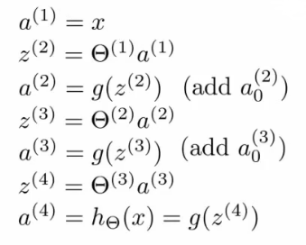
For a single training example $(x, y)$, forward propagation proceeds as follows:

• Layer 1 (Input): $a^{(1)} = x$
• Layer 2 (Hidden): $z^{(2)} = \Theta^{(1)} a^{(1)} \implies a^{(2)} = g(z^{(2)})$ (add bias unit $a_0^{(2)} = 1$)
• Layer 3 (Hidden): $z^{(3)} = \Theta^{(2)} a^{(2)} \implies a^{(3)} = g(z^{(3)})$ (add bias unit $a_0^{(3)} = 1$)
• Layer 4 (Output): $z^{(4)} = \Theta^{(3)} a^{(3)} \implies a^{(4)} = g(z^{(4)}) = h_\Theta(x)$

What is Backpropagation?

Backpropagation calculates an error term $\delta_j^{(l)}$ for each node $j$ in layer $l$. Intuitively, $\delta_j^{(l)}$ measures the "error" in the activation $a_j^{(l)}$ of unit $j$ in layer $l$.

Since $a_j^{(l)}$ is an activation computed by the network, we evaluate how far off it is relative to the target:

• The only ground truth target we have is the true label $y$ at the output layer $L$.
• For the output layer ($L = 4$ in our example), the error vector $\delta^{(4)}$ is simply:

In vectorized form:

Next, we propagate these errors backward to compute the error vectors for hidden layers:

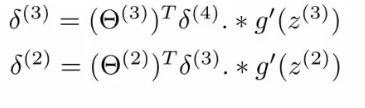
Where:

• $\odot$ denotes element-wise (pairwise) multiplication (in Octave/MATLAB, .*).
• $g'(z^{(l)})$ is the derivative of the sigmoid activation function evaluated at $z^{(l)}$.
• Calculus shows that $g'(z^{(l)}) = a^{(l)} \odot (1 - a^{(l)})$.

Thus:

Note that there is no $\delta^{(1)}$ term because layer 1 is the input layer, which corresponds to actual features with zero error.

Analyzing Vector Dimensions

Let's check the matrix dimensions in our 4-layer example network ($s_1=3, s_2=5, s_3=5, s_4=4$):

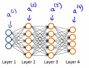
• $\Theta^{(3)}$ has size $[4 \times 5]$ (excluding bias column; $[4 \times 6]$ including bias column).
• $(\Theta^{(3)})^T$ has size $[5 \times 4]$.
• $\delta^{(4)}$ has size $[4 \times 1]$.
• Multiplying $(\Theta^{(3)})^T \delta^{(4)}$ yields a $[5 \times 1]$ vector.
• This matches the dimension of $a^{(3)}$ ($[5 \times 1]$), allowing element-wise multiplication $\odot$.

Why Do We Compute Delta Terms?

Through mathematical derivation, if we ignore regularization ($\lambda = 0$), the partial derivative for a single training example is simply:

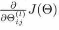
By computing the activation values $a_j^{(l)}$ during forward propagation and error terms $\delta_i^{(l+1)}$ during backpropagation, we get the partial derivative terms needed for gradient descent!

Complete Algorithm: Computing Partial Derivatives for $m$ Examples

Given a training set of $m$ examples:

We compute partial derivatives using an accumulator matrix $\Delta^{(l)}$ for each layer $l$:

1. Initialize Accumulators:

Set $\Delta_{ij}^{(l)} = 0$ for all $l, i, j$. (These matrices will accumulate gradients across examples).

2. Loop Over Training Examples:

For $i = 1$ to $m$:

• Set input activation $a^{(1)} = x^{(i)}$.
• Run forward propagation to compute activations $a^{(l)}$ for $l = 2, 3, \dots, L$.
• Compute output error vector: $\delta^{(L)} = a^{(L)} - y^{(i)}$.
• Run backpropagation to compute $\delta^{(L-1)}, \delta^{(L-2)}, \dots, \delta^{(2)}$.
• Accumulate the gradients:

In vectorized form:

3. Compute Final Gradient Matrices $D^{(l)}$:

After exiting the loop over all $m$ examples, compute the gradient terms $D_{ij}^{(l)}$:

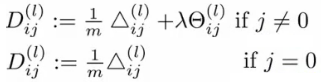
• For $j = 0$ (bias term, no regularization):

• For $j \ge 1$ (with regularization):

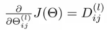
Once computed, each term $D_{ij}^{(l)}$ is exact:

These values are then passed into gradient descent or advanced optimization routines!

Backpropagation Intuition

Let's break down backpropagation step-by-step to gain visual intuition for how errors flow backward through the network.

Visualizing Forward Propagation

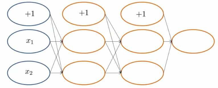
Consider a training example $(x^{(i)}, y^{(i)})$ with 2 input features ($x_1, x_2$). Forward propagation passes activations forward:

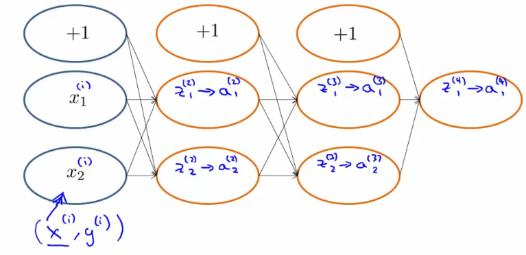
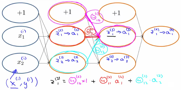
Each hidden node calculates a weighted sum of inputs $z_j^{(l)}$:

Applying the sigmoid function $g(z)$ yields the activation $a_1^{(2)} = g(z_1^{(2)})$:

Visualizing Backpropagation

For a single output binary classification problem, the cost for a single example $(x^{(i)}, y^{(i)})$ simplifies to:

Conceptually, this measures how well the network performs on example $i$. You can think of it as a sigmoidal version of squared error $(h_\Theta(x) - y)^2$.

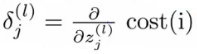
Formally, the delta term $\delta_j^{(l)}$ represents the partial derivative of the cost with respect to the weighted input sum $z_j^{(l)}$:

Error Propagation

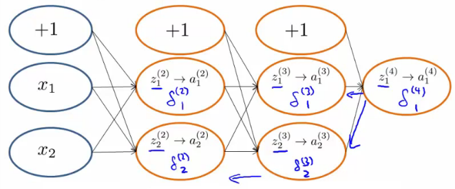
1. At the output layer, $\delta_1^{(4)} = a_1^{(4)} - y^{(1)}$ is the difference between predicted activation and actual target.
2. Going backward, node error $\delta_j^{(l)}$ is calculated as the weighted sum of errors from the next layer's nodes, weighted by the parameter links connecting them:

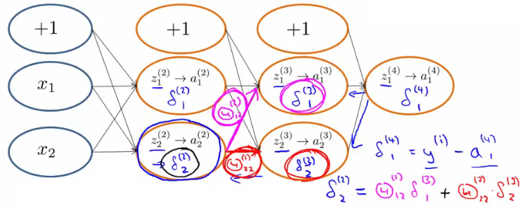
Thus, forward propagation computes activation values moving left-to-right, while backpropagation computes error terms moving right-to-left.

Implementation Details: Unrolling Parameters

When using advanced optimization routines in MATLAB/Octave (such as fminunc), the cost function and initial parameter values must be passed as 1D vectors:

However, in neural networks, our parameters $\Theta^{(1)}, \Theta^{(2)}, \dots$ and gradients $D^{(1)}, D^{(2)}, \dots$ are matrices:

Unrolling and Reshaping Matrices in Octave

Suppose we have a 3-layer neural network with:

• $s_1 = 10$ input units
• $s_2 = 10$ hidden units
• $s_3 = 1$ output unit

The parameter matrix dimensions are:

• $\Theta^{(1)} \in \mathbb{R}^{10 \times 11}$
• $\Theta^{(2)} \in \mathbb{R}^{10 \times 11}$
• $\Theta^{(3)} \in \mathbb{R}^{1 \times 11}$

To convert these matrices into a single unrolled vector for fminunc:

% Unroll matrices into a single vector
thetaVec = [ Theta1(:); Theta2(:); Theta3(:) ];
DVec     = [ D1(:);     D2(:);     D3(:) ];

To reshape the vector back into matrices inside your cost function:

% Reshape unrolled vector back into parameter matrices
Theta1 = reshape(thetaVec(1:110), 10, 11);
Theta2 = reshape(thetaVec(111:220), 10, 11);
Theta3 = reshape(thetaVec(221:231), 1, 11);

Gradient Checking

Backpropagation is complex and subtle. A small bug in backpropagation can lead to a situation where $J(\Theta)$ appears to decrease during gradient descent, but fails to reach a true optimum.

To ensure our backpropagation implementation is 100% bug-free, we use gradient checking.

Numerical Gradient Estimation

Consider a scalar function $J(\theta)$ where $\theta \in \mathbb{R}$. We can estimate the derivative numerically using the two-sided difference:

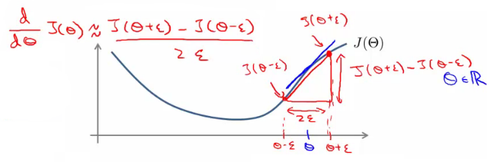
Typically, $\epsilon$ is chosen to be small, e.g., $\epsilon = 10^{-4}$.

For a parameter vector $\Theta \in \mathbb{R}^n$, we approximate the partial derivative with respect to each parameter $\theta_i$:

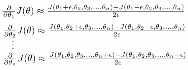
Octave Implementation of Gradient Checking

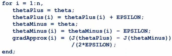
for i = 1:n
  thetaPlus = theta;
  thetaPlus(i) = thetaPlus(i) + EPSILON;
  
  thetaMinus = theta;
  thetaMinus(i) = thetaMinus(i) - EPSILON;
  
  gradApprox(i) = (J(thetaPlus) - J(thetaMinus)) / (2 * EPSILON);
end

Gradient Checking Protocol

1. Implement backpropagation to compute the analytical gradient vector DVec.
2. Implement numerical gradient checking to compute gradApprox.
3. Verify that gradApprox $\approx$ DVec to several decimal places.
4. IMPORTANT: Turn off gradient checking before running learning algorithms to train the model!

Warning: Numerical gradient checking is computationally very expensive because it requires evaluating $J(\Theta)$ twice for every single parameter. Backpropagation is far faster and should be used for actual training.

Random Initialization

For linear regression or logistic regression, initializing parameters $\Theta = \mathbf{0}$ (all zeros) works fine. However, zero initialization fails completely for neural networks.

The Symmetry Problem

If all weights are initialized to zero:

• Every hidden unit in layer $l$ will compute the exact same activation $a_j^{(l)}$.
• Every hidden unit will receive the exact same error $\delta_j^{(l)}$.
• Every weight will undergo identical updates during gradient descent ($\frac{\partial}{\partial \Theta_{ij}^{(l)}} J(\Theta)$ will be identical across units).
• The hidden units remain symmetrical and fail to learn distinct features.

Random Initialization Solution (Symmetry Breaking)

To break symmetry, initialize each weight $\Theta_{ij}^{(l)}$ randomly to a small value in $[-\epsilon_{init}, \epsilon_{init}]$:

% Initialize weights randomly in [-epsilon_init, epsilon_init]
Theta1 = rand(10, 11) * (2 * EPSILON_INIT) - EPSILON_INIT;
Theta2 = rand(10, 11) * (2 * EPSILON_INIT) - EPSILON_INIT;
Theta3 = rand(1, 11)  * (2 * EPSILON_INIT) - EPSILON_INIT;

Putting It All Together

Here is a step-by-step guide to designing and training a neural network.

Step 1: Select Network Architecture

Pick a network layout (connectivity structure between neurons):

• Input units: $n = \text{dimension of feature vector } x^{(i)}$.
• Output units: $K = \text{number of classes}$.
  • Binary classification: 1 output unit.
  • Multi-class classification: $K$ output units (one-hot vector).
• Hidden layers:
  • Default: 1 hidden layer.
  • If using multiple hidden layers, recommended to have the same number of hidden units in each hidden layer.
  • Number of hidden units: usually equal to or 1.5–2$\times$ the number of input features. More hidden units generally improve representation capacity but increase computational cost.

Step 2: Training a Neural Network

1. Randomly initialize weights: Small random values near zero (e.g., in $[-\epsilon_{init}, \epsilon_{init}]$).
2. Implement forward propagation: Compute $h_\Theta(x^{(i)})$ for any input $x^{(i)}$.
3. Implement cost function code: Compute $J(\Theta)$.
4. Implement backpropagation: Compute partial derivative terms $\frac{\partial}{\partial \Theta_{ij}^{(l)}} J(\Theta)$.

% General loop over training set for backpropagation
for i = 1:m
  % 1. Forward propagation on (x^i, y^i) to get activation (a) terms
  % 2. Backpropagation on (x^i, y^i) to get error (delta) terms
  % 3. Accumulate delta: Delta^(l) := Delta^(l) + delta^(l+1) * (a^(l))'
end

% Compute final D matrix partial derivatives with regularization

5. Perform gradient checking: Compare $D^{(l)}$ with numerical gradient approximation gradApprox. Disable gradient checking once confirmed working!
6. Minimize $J(\Theta)$: Use gradient descent or advanced optimization algorithms (e.g., fminunc, L-BFGS) with backpropagation to minimize $J(\Theta)$ as a function of parameters $\Theta$.

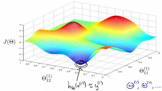
Note on Non-Convexity: For neural networks, the cost function $J(\Theta)$ is non-convex and can theoretically get stuck in local minima. In practice, gradient descent algorithms initialized with small random weights find very effective local (or global) minima.