Lecture 08: Neural Networks - Representation

Non-linear Hypotheses

Why Do We Need Neural Networks?

Consider a complex supervised classification problem. We could attempt to use logistic regression with many polynomial terms:

• Works well when you have only $1$ or $2$ features.
• However, if you have $100$ features (e.g., predicting the probability of a house selling in the next 6 months based on 100 features of the house), including all quadratic (second-order) terms: $x_1^2, x_1 x_2, x_1 x_3, \dots, x_1 x_{100}, x_2^2, x_2 x_3, \dots, x_{100}^2$ results in approximately $5,000$ features for $n = 100$.

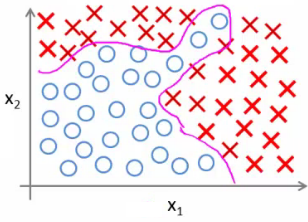
The number of quadratic features grows on the order of $O(n^2)$:

• For $n = 100$, feature count $\approx \frac{n^2}{2} \approx 5,000$.
• Working with this many features is computationally expensive.
• Simply selecting a small subset of features often leaves the model unable to fit a complex dataset adequately.

If we include cubic (third-order) terms (e.g., $x_1^2 x_2, x_1 x_2 x_3, x_1 x_4 x_{23}$):

• The number of features grows on the order of $O(n^3)$.
• For $n = 100$, there are approximately $170,000$ features.
• Consequently, polynomial logistic regression becomes impractical when $n$ is large.

Example: Problems Where $n$ is Large (Computer Vision)

Computer vision algorithms process images as matrices of pixel intensity values.

To build a car detector:

1. Collect a training set of images containing cars ($y = 1$) and not cars ($y = 0$).
2. Test an unseen image to classify whether it contains a car.

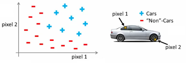
To understand why this is challenging:

• Suppose we select two specific pixel locations and plot their intensity values. We need a non-linear decision boundary to separate the two classes in feature space.
• For a small $50 \times 50$ pixel grayscale image, there are $n = 2,500$ pixels.
• Including all quadratic features $(x_i x_j)$ yields approximately $3 \times 10^6$ features.
• If using RGB images, $n = 7,500$, yielding tens of millions of features.
• For a $100 \times 100$ RGB image, $n = 30,000$, resulting in hundreds of millions of features.

Thus, standard logistic regression with polynomial features is unsuitable for high-dimensional complex data. Neural networks provide a much more effective framework for learning non-linear hypotheses in huge feature spaces.

Neurons and the Brain

Neural networks (NNs) were originally motivated by the desire to build algorithms that replicate the computational functionality of the biological brain.

• Origins: Developed extensively in the 1980s and 1990s. Popularity waned in the late 1990s due to computational constraints, but saw a massive resurgence as modern computing hardware made training large-scale networks computationally feasible.
• The "One Learning Algorithm" Hypothesis: Evidence suggests the brain may use a single master learning algorithm for diverse sensory inputs.
  • Neuroplasticity experiments: Re-routing the optic nerve to the auditory cortex (sound processing region) enables the auditory cortex to learn to process visual signals ("learns to see"). Re-routing to the somatosensory cortex yields similar results.
• Human-Machine Interface Examples:
  • BrainPort: A camera feeds pixel data to a grid of electrodes on the tongue, allowing visually impaired individuals to perceive visual patterns through tactile tongue stimulation.
  • Human Echolocation: Training individuals to navigate environments by interpreting acoustic reflections.
  • Haptic Direction Belts: A belt that pulses in the direction of magnetic north, giving users a continuous sensory orientation.

---

Model Representation I

How Do We Represent Neural Networks?

Neural networks were designed to simulate networks of biological neurons.

A biological neuron consists of three main structural parts:

1. Cell body: Performs cellular computations.
2. Dendrites: Input wires that receive electrical signals from other neurons.
3. Axon: Output wire that transmits electrical pulses (spikes) to other neurons.

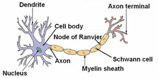
At a high level:

• A neuron receives inputs via dendrites.
• Performs processing in the cell body.
• Sends output pulses down the axon to downstream neurons.

Artificial Neural Network - Representation of a Neuron

In an artificial neural network, a neuron is modeled as a logistic unit:

• Inputs $x_1, x_2, x_3$ are fed in via input wires.
• The unit evaluates a logistic computation.
• Sends output $h_\theta(x)$ down output wires.

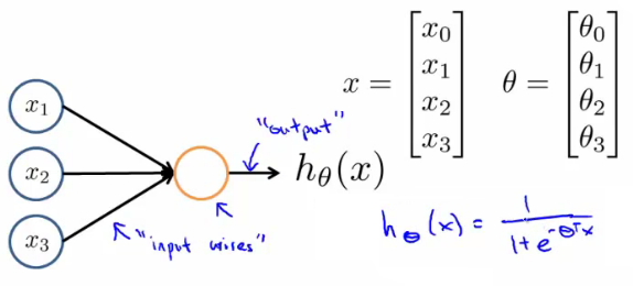
An additional bias unit $x_0 = 1$ is often included. The parameters $\theta = [\theta_0, \theta_1, \theta_2, \theta_3]^T$ are referred to as the weights of the model:

$h_\theta(x) = \frac{1}{1 + e^{-\theta^T x}}$

Where the activation function $g(z)$ is the sigmoid (logistic) function: $g(z) = \frac{1}{1 + e^{-z}}$

Neural Network Architecture

When multiple artificial neurons are connected together, they form a neural network:

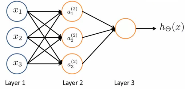
The network is organized into layers:

• Layer 1 (Input Layer): Contains input features $x_1, x_2, x_3$ (plus bias unit $x_0 = 1$).
• Layer 2 (Hidden Layer): Middle layer containing hidden activation units $a_1^{(2)}, a_2^{(2)}, a_3^{(2)}$ (plus bias unit $a_0^{(2)} = 1$). "Hidden" indicates that these values are intermediate computation steps not directly observed in the training set.
• Layer 3 (Output Layer): Produces the final computed value $h_\theta(x) = a_1^{(3)}$.

Neural Network Notation

• $a_i^{(j)}$: Activation of unit $i$ in layer $j$ (the value computed and output by node $i$ in layer $j$).
• $\Theta^{(j)}$: Matrix of parameters (weights) controlling the function mapping from layer $j$ to layer $j + 1$.

Matrix Dimensions Rule:

If a network has $s_j$ units in layer $j$ and $s_{j+1}$ units in layer $j + 1$, then the weight matrix $\Theta^{(j)}$ has dimensions: $\Theta^{(j)} \in \mathbb{R}^{s_{j+1} \times (s_j + 1)}$

• Number of rows ($s_{j+1}$): Equal to the number of units in layer $j + 1$.
• Number of columns ($s_j + 1$): Equal to the number of units in layer $j$ plus $1$ (for the bias unit).

Example: If Layer 1 has 10 input units and Layer 2 has 20 hidden units, $\Theta^{(1)}$ will have dimensions $[20 \times 11]$.

Layer Computations

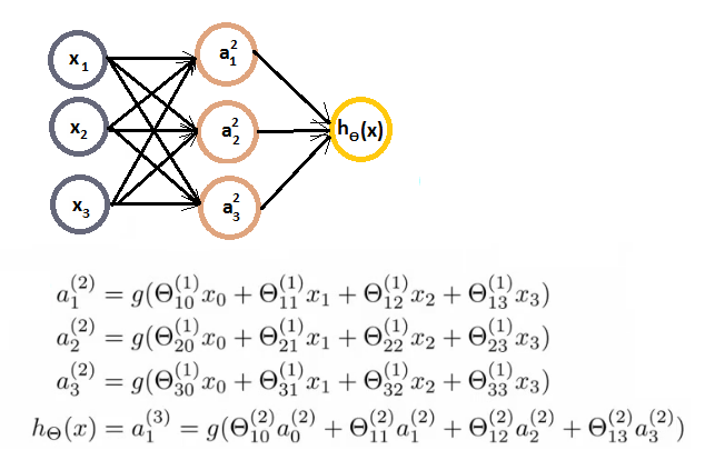
For the 3-layer architecture shown above, the activations of the hidden units in Layer 2 are calculated as:

$a_1^{(2)} = g\left(\Theta_{10}^{(1)} x_0 + \Theta_{11}^{(1)} x_1 + \Theta_{12}^{(1)} x_2 + \Theta_{13}^{(1)} x_3\right)$ $a_2^{(2)} = g\left(\Theta_{20}^{(1)} x_0 + \Theta_{21}^{(1)} x_1 + \Theta_{22}^{(1)} x_2 + \Theta_{23}^{(1)} x_3\right)$ $a_3^{(2)} = g\left(\Theta_{30}^{(1)} x_0 + \Theta_{31}^{(1)} x_1 + \Theta_{32}^{(1)} x_2 + \Theta_{33}^{(1)} x_3\right)$

The final hypothesis output in Layer 3 is computed using the activation values from Layer 2:

$h_\theta(x) = a_1^{(3)} = g\left(\Theta_{10}^{(2)} a_0^{(2)} + \Theta_{11}^{(2)} a_1^{(2)} + \Theta_{12}^{(2)} a_2^{(2)} + \Theta_{13}^{(2)} a_3^{(2)}\right)$

Where $a_0^{(2)} = 1$ is the bias unit added to Layer 2.

Parameter Indexing Notation:

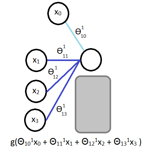
In general, parameter element $\Theta_{j i}^{(l)}$ represents:

• $l$: The layer mapping FROM (layer $l \to \text{layer } l+1$).
• $j$: The destination unit index in layer $l+1$.
• $i$: The source unit index in layer $l$.

Example: $\Theta_{1 3}^{(1)}$ controls the mapping from unit $3$ in Layer 1 to unit $1$ in Layer 2.

---

Model Representation II

Vectorized Implementation of Forward Propagation

To perform computations efficiently, we vectorize the step-by-step activations.

Define intermediate linear values $z_i^{(j)}$ as the weighted inputs to activation function $g$: $z_1^{(2)} = \Theta_{10}^{(1)} x_0 + \Theta_{11}^{(1)} x_1 + \Theta_{12}^{(1)} x_2 + \Theta_{13}^{(1)} x_3$ $z_2^{(2)} = \Theta_{20}^{(1)} x_0 + \Theta_{21}^{(1)} x_1 + \Theta_{22}^{(1)} x_2 + \Theta_{23}^{(1)} x_3$ $z_3^{(2)} = \Theta_{30}^{(1)} x_0 + \Theta_{31}^{(1)} x_1 + \Theta_{32}^{(1)} x_2 + \Theta_{33}^{(1)} x_3$

Thus, each activation is $a_i^{(2)} = g(z_i^{(2)})$.

Define vectors:

$$$$

Vectorizing the calculation of Layer 2: $z^{(2)} = \Theta^{(1)} x$ $a^{(2)} = g(z^{(2)})$

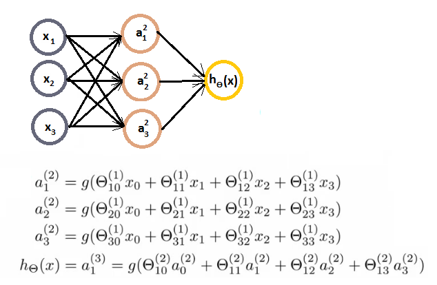
Where:

• $\Theta^{(1)}$ is a $[3 \times 4]$ matrix.
• $x$ is a $[4 \times 1]$ vector.
• $z^{(2)}$ and $a^{(2)}$ are $[3 \times 1]$ vectors.
• $g(\cdot)$ applies the sigmoid function element-wise to vector $z^{(2)}$.

To keep notation consistent across layers, define the input layer vector as $a^{(1)} = x$: $z^{(2)} = \Theta^{(1)} a^{(1)}$ $a^{(2)} = g(z^{(2)})$

To calculate the output layer, add a bias unit $a_0^{(2)} = 1$ to $a^{(2)}$, expanding $a^{(2)}$ into a $[4 \times 1]$ vector.

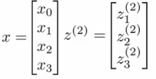
Then compute $z^{(3)}$ and the final hypothesis: $z^{(3)} = \Theta^{(2)} a^{(2)}$ $h_\theta(x) = a^{(3)} = g(z^{(3)})$

This process of starting with the input layer activations $a^{(1)} = x$ and sequentially calculating activations layer-by-layer forward through the network is called Forward Propagation.

Neural Networks Learning Its Own Features

Consider the final output layer (Layer 3) of our network:

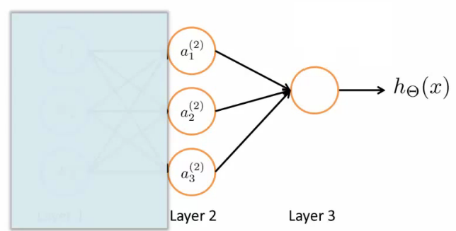
The hypothesis function evaluates as: $h_\theta(x) = g\left(\Theta_{10}^{(2)} a_0^{(2)} + \Theta_{11}^{(2)} a_1^{(2)} + \Theta_{12}^{(2)} a_2^{(2)} + \Theta_{13}^{(2)} a_3^{(2)}\right)$

Notice that this is identical to standard logistic regression! The critical difference is:

• Standard logistic regression performs classification directly on raw input features $x_1, x_2, x_3$.
• A neural network performs classification using learned features $a_1^{(2)}, a_2^{(2)}, a_3^{(2)}$ calculated by the hidden layer mapping $\Theta^{(1)}$.

Instead of manually engineering high-order polynomial features, the neural network automatically learns optimal non-linear feature representations in its hidden layers to feed into the final logistic regression output node.

Network Architecture Variations

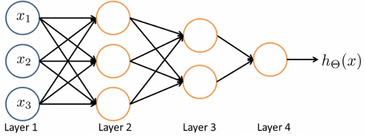
Neural networks can be configured with various topologies depending on problem complexity:

• Different numbers of hidden units per layer.
• Multiple hidden layers (e.g., Layer 2 and Layer 3 as hidden layers, with Layer 4 as output).

---

Neural Network Example: Computing Complex Non-linear Functions

To gain intuition for how neural networks compute complex non-linear decision boundaries, we can construct networks for basic boolean logical functions.

Non-linear Classification: XOR / XNOR

Consider binary inputs $x_1, x_2 \in \{0, 1\}$. We want to learn a non-linear decision boundary for the XNOR function: $y = x_1 \text{ XNOR } x_2 = \text{NOT } (x_1 \text{ XOR } x_2)$

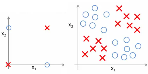
• Positive instances $(y = 1)$: $(0, 0)$ and $(1, 1)$.
• Negative instances $(y = 0)$: $(0, 1)$ and $(1, 0)$.

Example 1: Logical AND Function

Can a single artificial neuron compute the logical AND function?

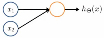
Set up a neuron with inputs $x_1, x_2$ and bias $x_0 = 1$. Assign weights:

$$$$

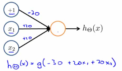
The hypothesis equation is: $h_\theta(x) = g(-30 + 20x_1 + 20x_2)$

Evaluating all four binary input combinations:

Thus, $h_\theta(x) \approx x_1 \text{ AND } x_2$.

Example 2: Logical OR Function

Set up a neuron with weights:

$$$$

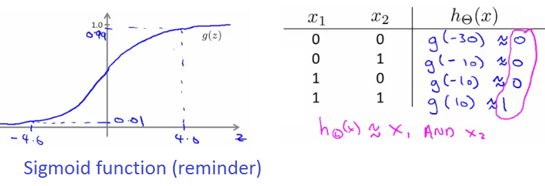
The hypothesis equation is: $h_\theta(x) = g(-10 + 20x_1 + 20x_2)$

Evaluating input combinations:

Thus, $h_\theta(x) \approx x_1 \text{ OR } x_2$.

Example 3: Logical NOT and NOR Functions

To perform negation (NOT $x_1$), place a large negative weight in front of input variable $x_1$:

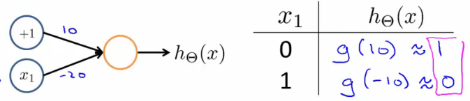
With weights $\Theta^{(1)} = \begin{bmatrix} 10 & -20 \end{bmatrix}$: $h_\theta(x) = g(10 - 20x_1)$

• $x_1 = 0 \implies g(10) \approx 1$
• $x_1 = 1 \implies g(-10) \approx 0$

To compute $(\text{NOT } x_1) \text{ AND } (\text{NOT } x_2)$ (NOR gate), use weights:

$$$$

$h_\theta(x) = g(10 - 20x_1 - 20x_2)$

• $x_1=0, x_2=0 \implies g(10) \approx 1$
• Any input of 1 yields $g(-10) \approx 0$ or $g(-30) \approx 0$.

Combining Gates: XNOR Circuit

We can combine logical AND, NOR, and OR gates into a 2-layer neural network to compute $x_1 \text{ XNOR } x_2$:

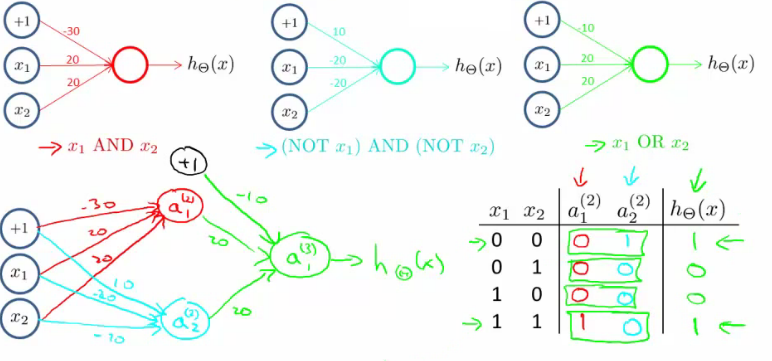
Layer 2 (Hidden Layer):

• Node $a_1^{(2)}$ computes $x_1 \text{ AND } x_2$: $a_1^{(2)} = g(-30 + 20x_1 + 20x_2)$
• Node $a_2^{(2)}$ computes $(\text{NOT } x_1) \text{ AND } (\text{NOT } x_2)$: $a_2^{(2)} = g(10 - 20x_1 - 20x_2)$

Layer 3 (Output Layer):

• Node $a_1^{(3)}$ combines hidden activations using an OR gate: $a_1^{(3)} = g(-10 + 20a_1^{(2)} + 20a_2^{(2)})$

Truth Table Evaluation:

By layering simple linear units, neural networks can build up complex non-linear functions step-by-step.

Practical Application: Handwritten Digit Recognition

Machine learning pioneer Yann LeCun developed early multi-layer neural networks (LeNet) for automated zip code and handwritten digit recognition on postal envelopes. By training hierarchical layers to detect edges, strokes, and digits, these networks achieved commercial success long before the deep learning era.

---

Multiclass Classification

Multiclass classification involves distinguishing between more than two categories ($K > 2$), such as recognizing digits ($0-9$) or identifying four object classes: Pedestrian, Car, Motorcycle, and Truck.

One-vs-All Extension for Neural Networks

To classify $K$ classes, construct a neural network with $K$ output nodes in the final layer:

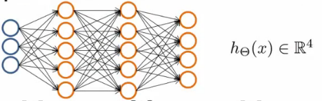
For a 4-class problem ($K = 4$), the output layer yields a 4-dimensional vector: $h_\theta(x) \in \mathbb{R}^4$

Where each output node estimates the probability of belonging to one specific class:

• $h_\theta(x)_1 = P(y = 1 \mid x)$ (Pedestrian)
• $h_\theta(x)_2 = P(y = 2 \mid x)$ (Car)
• $h_\theta(x)_3 = P(y = 3 \mid x)$ (Motorcycle)
• $h_\theta(x)_4 = P(y = 4 \mid x)$ (Truck)

Target Output Representation ($y$)

Instead of representing target label $y$ as a single scalar integer $\{1, 2, 3, 4\}$, represent $y^{(i)}$ as a one-hot vector:

$$y^{(i)} \in \left\{ \begin{bmatrix} 1 \\ 0 \\ 0 \\ 0 \end{bmatrix}, \begin{bmatrix} 0 \\ 1 \\ 0 \\ 0 \end{bmatrix}, \begin{bmatrix} 0 \\ 0 \\ 1 \\ 0 \end{bmatrix}, \begin{bmatrix} 0 \\ 0 \\ 0 \\ 1 \end{bmatrix} \right\}$$

• For a Pedestrian image: $y^{(i)} = \begin{bmatrix} 1 \\ 0 \\ 0 \\ 0 \end{bmatrix}$
• For a Car image: $y^{(i)} = \begin{bmatrix} 0 \\ 1 \\ 0 \\ 0 \end{bmatrix}$
• For a Motorcycle image: $y^{(i)} = \begin{bmatrix} 0 \\ 0 \\ 1 \\ 0 \end{bmatrix}$
• For a Truck image: $y^{(i)} = \begin{bmatrix} 0 \\ 0 \\ 0 \\ 1 \end{bmatrix}$

During training, the goal is to optimize network parameters $\Theta$ such that: $h_\theta(x^{(i)}) \approx y^{(i)}$