Lecture 12: Support Vector Machines

Support Vector Machine (SVM) - Optimization Objective

• So far, we've seen a range of different algorithms
  • With supervised learning algorithms - performance is pretty similar
    • What matters more often is;
      • The amount of training data
      • Skill of applying algorithms
• One final supervised learning algorithm that is widely used - support vector machine (SVM)
• Compared to both logistic regression and neural networks, a SVM sometimes gives a cleaner way of learning non-linear functions
• Later in the course we'll do a survey of different supervised learning algorithms

An Alternative View of Logistic Regression

• Start with logistic regression, see how we can modify it to get the SVM
  • As before, the logistic regression hypothesis is as follows

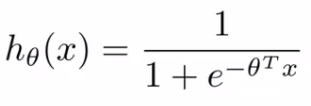
• And the sigmoid activation function looks like this

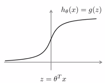
• In order to explain the math, we use z as defined above
• What do we want logistic regression to do?
  • We have an example where y = 1
    • Then we hope $h_\theta(x)$ is close to 1
    • With $h_\theta(x)$ close to 1, $\theta^T x$ must be much larger than 0

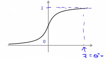
• Similarly, when y = 0
  • Then we hope $h_\theta(x)$ is close to 0
  • With $h_\theta(x)$ close to 0, $\theta^T x$ must be much less than 0
• This is our classic view of logistic regression
  • Let's consider another way of thinking about the problem
• Alternative view of logistic regression
  • If you look at cost function, each example contributes a term like the one below to the overall cost function

• For the overall cost function, we sum over all the training examples using the above function, and have a $\frac{1}{m}$ term
• If you then plug in the hypothesis definition ($h_\theta(x)$), you get an expanded cost function equation;

• So each training example contributes that term to the cost function for logistic regression

• If y = 1 then only the first term in the objective matters

  • If we plot the functions vs. z we get the following graph

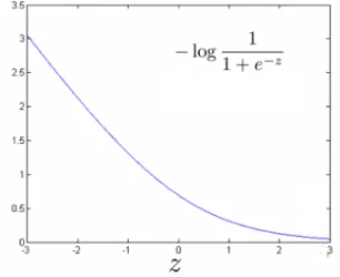
• This plot shows the cost contribution of an example when y = 1 given z
  • So if z is big, the cost is low - this is good!
  • But if z is 0 or negative the cost contribution is high
  • This is why, when logistic regression sees a positive example, it tries to set $\theta^T x$ to be a very large term
• If y = 0 then only the second term matters
• We can again plot it and get a similar graph

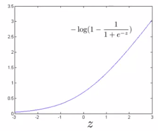
• Same deal, if z is small then the cost is low
  • But if s is large then the cost is massive

SVM Cost Functions from Logistic Regression Cost Functions

• To build a SVM we must redefine our cost functions
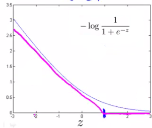
  • When y = 1
    • Take the y = 1 function and create a new cost function
    • Instead of a curved line create two straight lines (magenta) which acts as an approximation to the logistic regression y = 1 function

• Take point (1) on the z axis

  • Flat from 1 onwards
  • Grows when we reach 1 or a lower number

• This means we have two straight lines

  • Flat when cost is 0
  • Straight growing line after 1

• So this is the new y=1 cost function

  • Gives the SVM a computational advantage and an easier optimization problem
  • We call this function $\text{cost}_1(z)$

• Similarly

  • When y = 0
    • Do the equivalent with the y=0 function plot

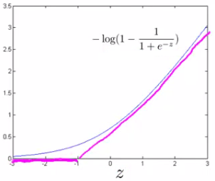
• We call this function $\text{cost}_0(z)$
• So here we define the two cost function terms for our SVM graphically
  • How do we implement this?

The Complete SVM Cost Function

• As a comparison/reminder we have logistic regression below

• If this looks unfamiliar its because we previously had the - sign outside the expression
• For the SVM we take our two logistic regression y=1 and y=0 terms described previously and replace with
  • $\text{cost}_1(\theta^T x)$
  • $\text{cost}_0(\theta^T x)$
• So we get

SVM Notation is Slightly Different

• In convention with SVM notation we rename a few things here
• 1) Get rid of the $\frac{1}{m}$ terms
  • This is just a slightly different convention
  • By removing $\frac{1}{m}$ we should get the same optimal values for
    • $\frac{1}{m}$ is a constant, so should get same optimization
    • e.g. say you have a minimization problem which minimizes to u = 5
      • If your cost function * by a constant, you still generates the minimal value
      • That minimal value is different, but that's irrelevant
• 2) For logistic regression we had two terms;
  • Training data set term (i.e. that we sum over m) = A
  • Regularization term (i.e. that we sum over n) = B
    • So we could describe it as A + $\lambda$B
    • Need some way to deal with the trade-off between regularization and data set terms
    • Set different values for $\lambda$ to parametrize this trade-off
  • Instead of parameterization this as A + $\lambda$B
    • For SVMs the convention is to use a different parameter called C
    • So do CA + B
    • If C were equal to 1/$\lambda$ then the two functions (CA + B and A + $\lambda$B) would give the same value
• So, our overall equation is

• Unlike logistic, $h_\theta(x)$ doesn't give us a probability, but instead we get a direct prediction of 1 or 0
• So if $\theta^T x$ is equal to or greater than 0 --> $h_\theta(x)$ = 1
• Else --> $h_\theta(x)$ = 0

Large Margin Intuition

• Sometimes people refer to SVM as large margin classifiers
  • We'll consider what that means and what an SVM hypothesis looks like
  • The SVM cost function is as above, and we've drawn out the cost terms below

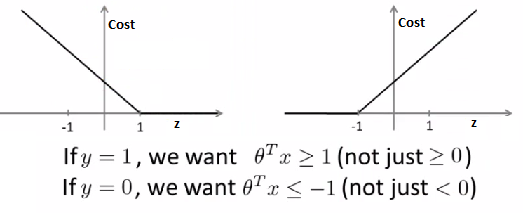
• Left is cost_1 and right is cost_0
• What does it take to make terms small
  • If y =1
    • $\text{cost}_1(z)$ = 0 only when z >= 1
  • If y = 0
    • $\text{cost}_0(z) = 0$ only when $z \le -1$
• Interesting property of SVM
  • If you have a positive example, you only really need z to be greater or equal to 0
    • If this is the case then you predict 1
  • SVM wants a bit more than that - doesn't want to just get it right, but have the value be quite a bit bigger than zero
    • Throws in an extra safety margin factor
• Logistic regression does something similar
• What are the consequences of this?
  • Consider a case where we set C to be huge
    • C = 100,000
    • So considering we're minimizing CA + B
      • If C is huge we're going to pick an A value so that A is equal to zero
      • What is the optimization problem here - how do we make A = 0?
    • Making A = 0
      • If y = 1
        • Then to make our "A" term 0 need to find a value of $\theta$ so $\theta^T x$ is greater than or equal to 1
      • Similarly, if y = 0
        • Then we want to make "A" = 0 then we need to find a value of $\theta$ so $\theta^T x$ is equal to or less than -1
    • So - if we think of our optimization problem a way to ensure that this first "A" term is equal to 0, we re-factor our optimization problem into just minimizing the "B" (regularization) term, because
      • When A = 0 --> A*C = 0
    • So we're minimizing B, under the constraints shown below

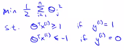
• Turns out when you solve this problem you get interesting decision boundaries

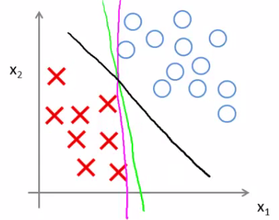
• The green and magenta lines are functional decision boundaries which could be chosen by logistic regression
  • But they probably don't generalize too well
• The black line, by contrast is the the chosen by the SVM because of this safety net imposed by the optimization graph
  • More robust separator
• Mathematically, that black line has a larger minimum distance (margin) from any of the training examples

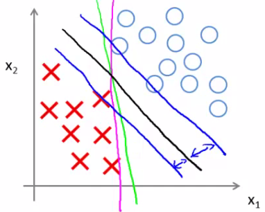
• By separating with the largest margin you incorporate robustness into your decision making process
• We looked at this at when C is very large
• SVM is more sophisticated than the large margin might look
  • If you were just using large margin then SVM would be very sensitive to outliers

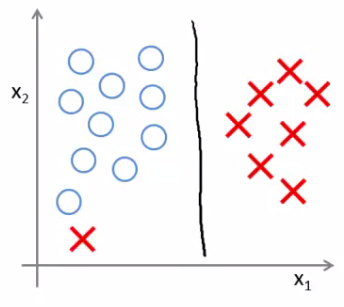
• You would risk making a ridiculous hugely impact your classification boundary
  • A single example might not represent a good reason to change an algorithm
  • If C is very large then we do use this quite naive maximize the margin approach

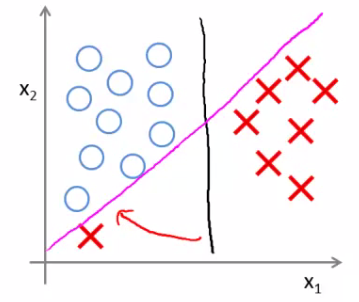
• So we'd change the black to the magenta
• But if C is reasonably small, or a not too large, then you stick with the black decision boundary
• What about non-linearly separable data?
  • Then SVM still does the right thing if you use a normal size C
  • So the idea of SVM being a large margin classifier is only really relevant when you have no outliers and you can easily linearly separable data
• Means we ignore a few outliers

Large Margin Classification Mathematics (Optional)

Vector Inner Products

• Have two (2D) vectors $u$ and $v$ - what is the inner product ($u^T v$)?

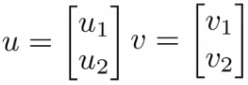
• Plot u on graph
  • i.e. $u_1$ vs. $u_2$

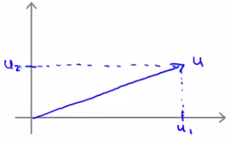
• One property which is good to have is the normof a vector
  • Written as $\|u\|$
    • This is the euclidean length of vector u
  • So $\|u\| = \sqrt{u_1^2 + u_2^2} = \text{real number}$
    • i.e. length of the arrow above
    • Can show via Pythagoras
• For the inner product, take v and orthogonally project down onto u
  • First we can plot v on the same axis in the same way (v_1vs v_1)
  • Measure the length/magnitude of the projection

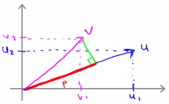
• So here, the green line is the projection
  • p = length along u to the intersection
  • p is the magnitude of the projection of vector v onto vector u
• Possible to show that
  • $u^T v = p \cdot \|u\|$
    • So this is one way to compute the inner product
  • $u^T v = u_1 v_1 + u_2 v_2$
  • So therefore
    • $p \cdot \|u\| = u_1 v_1 + u_2 v_2$
    • This is an important rule in linear algebra
  • We can reverse this too
    • So we could do
      • $v^T u = v_1 u_1 + v_2 u_2$
      • Which would obviously give you the same number
• p can be negative if the angle between them is 90 degrees or more

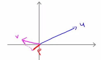
• So here p is negative
• Use the vector inner product theory to try and understand SVMs a little better

SVM Decision Boundary

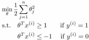
• For the following explanation - two simplification
  • Set $\theta_0 = 0$ (i.e., ignore intercept terms)
  • Set $n = 2$ (i.e., feature vector $(x_1, x_2)$)
    • i.e., each example has only 2 features
• Given we only have two parameters we can simplify our function to

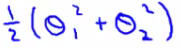
• And, can be re-written as

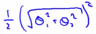
• Should give same thing
• We may notice that

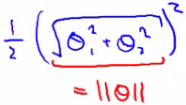
• The term in red is the norm of $\theta$
  • If we take $\theta$ as a 2x1 vector
  • If we assume $\theta_0$ = 0 its still true
• So, finally, this means our optimization function can be re-defined as

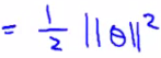
• So the SVM is minimizing the squared norm

• Given this, what are the $\theta^T x$ parameters doing?

  • Given $\theta$ and given example x what is this equal to
    • We can look at this in a comparable manner to how we just looked at u and v
  • Say we have a single positive training example (red cross below)

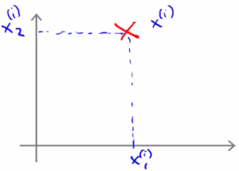
• Although we haven't been thinking about examples as vectors it can be described as such

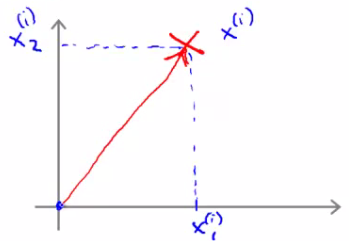
• Now, say we have our parameter vector $\theta$ and we plot that on the same axis

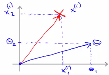
• The next question is what is the inner product of these two vectors

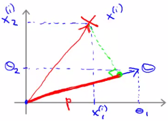
• p, is in fact p^i, because it's the length of p for example i
  • Given our previous discussion we know $\theta^T x^{(i)} = p^{(i)} \cdot \|\theta\|$

$= \theta_1 x_1^{(i)} + \theta_2 x_2^{(i)}$

• So these are both equally valid ways of computing $\theta^T x^{(i)}$
• What does this mean?
  • The constraints we defined earlier
    • $\theta^T x \ge 1$ if $y = 1$
    • $\theta^T x \le -1$ if $y = 0$
  • Can be replaced/substituted with the constraints
    • $p^{(i)} \cdot \|\theta\| \ge 1$ if $y = 1$
    • $p^{(i)} \cdot \|\theta\| \le -1$ if $y = 0$
• Writing that into our optimization objective

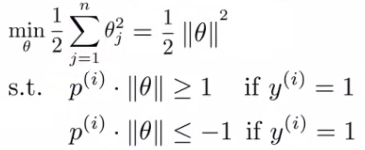
• So, given we've redefined these functions let us now consider the training example below

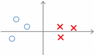
• Given this data, what boundary will the SVM choose? Note that we're still assuming $\theta_0$ = 0, which means the boundary has to pass through the origin (0,0)
  • Green line - small margins

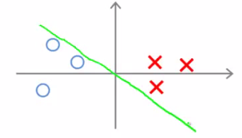
• SVM would not chose this line
  • Decision boundary comes very close to examples
  • Lets discuss why the SVM would not chose this decision boundary
• Looking at this line
  • We can show that $\theta$ is at 90 degrees to the decision boundary

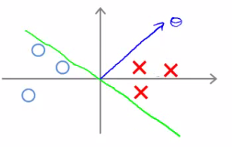
• $\theta$ is always at 90 degrees to the decision boundary (can show with linear algebra, although we're not going to!)
• So now lets look at what this implies for the optimization objective
  • Look at first example ($x^{(1)}$)

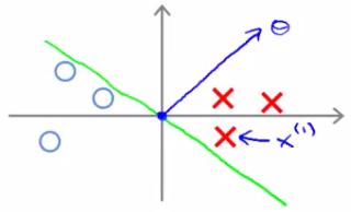
• Project a line from $x^{(1)}$ onto the $\theta$ vector (hitting at 90 degrees)
  • The distance between the intersection and the origin is $p^{(1)}$
• Similarly, look at second example ($x^{(2)}$)
• Project a line from $x^{(2)}$ onto the $\theta$ vector
• This is the magenta line, which will be negative ($p^{(2)}$)
• If we overview these two lines below we see a graphical representation of what's going on;

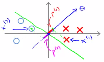
• We find that both these p values are going to be pretty small
• If we look back at our optimization objective
  • We know we need $p^{(1)} \cdot \|\theta\| \ge 1$ for positive examples
    • If p is small
      • Means that $\|\theta\|$ must be pretty large
  • Similarly, for negative examples we need p^2 * ||$\theta$|| to be smaller than or equal to -1
    • We saw in this example p^2 is a small negative number
      • So $\|\theta\|$ must be a large number
• Why is this a problem?
  • The optimization objective is trying to find a set of parameters where the norm of theta is small
    • So this doesn't seem like a good direction for the parameter vector (because as p values get smaller ||$\theta$|| must get larger to compensate)
      • So we should make p values larger which allows ||$\theta$|| to become smaller
• So lets chose a different boundary

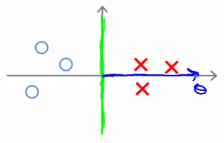
• Now if you look at the projection of the examples to $\theta$ we find that p^1becomes large and ||$\theta$|| can become small
• So with some values drawn in

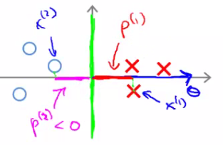
• This means that by choosing this second decision boundary we can make ||$\theta$|| smaller
  • Which is why the SVM choses this hypothesis as better
  • This is how we generate the large margin effect

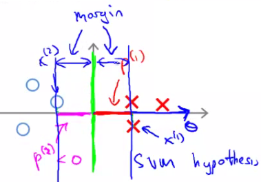
• The magnitude of this margin is a function of the p values
  • So by maximizing these p values we minimize ||$\theta$||
• Finally, we did this derivation assuming $\theta_0$ = 0,
  • If this is the case we're entertaining only decision boundaries which pass through (0,0)
  • If you allow $\theta_0$ to be other values then this simply means you can have decision boundaries which cross through the x and y values at points other than (0,0)
  • Can show with basically same logic that this works, and even when $\theta_0$ is non-zero when you have optimization objective described above (when C is very large) that the SVM is looking for a large margin separator between the classes

Kernels I: Adapting SVM to Non-Linear Classifiers

• What are kernels and how do we use them
  • We have a training set
  • We want to find a non-linear boundary

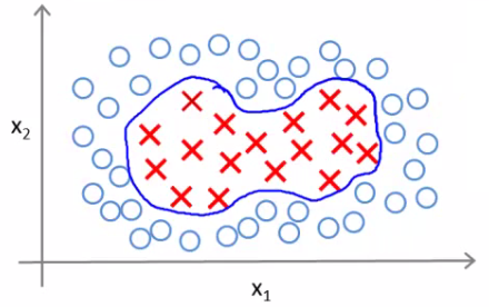
• Come up with a complex set of polynomial features to fit the data
  • Have $h_\theta(x)$ which
    • Returns 1 if the combined weighted sum of vectors (weighted by the parameter vector) is less than or equal to 0
    • Else return 0
  • Another way of writing this (new notation) is
    • That a hypothesis computes a decision boundary by taking the sum of the parameter vector multiplied by a new feature vector f, which simply contains the various high order x terms
    • e.g.
      • $h_\theta(x) = \theta_0 + \theta_1 f_1 + \theta_2 f_2 + \theta_3 f_3$
      • Where
        • $f_1 = x_1$
        • $f_2 = x_1 x_2$
        • $f_3 = \dots$
        • i.e. not specific values, but each of the terms from your complex polynomial function
  • Is there a better choice of feature f than the high order polynomials?
    • As we saw with computer imaging, high order polynomials become computationally expensive
• New features
• Define three features in this example (ignore x_0)
• Have a graph of $x_1$ vs. $x_2$ (don't plot the values, just define the space)
• Pick three points in that space

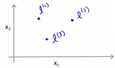
• These points $l^{(1)}, l^{(2)},$ and $l^{(3)}$ were chosen manually and are called landmarks
  • Given $x$, define $f_1$ as the similarity between $(x, l^{(1)})$
    • $= \exp\left( -\frac{\|x - l^{(1)}\|^2}{2\sigma^2} \right)$

=

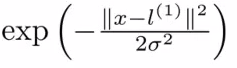
• $\|x - l^{(1)}\|$ is the Euclidean distance between point $x$ and landmark $l^{(1)}$ squared
  • Disussed more later
• If we remember our statistics, we know that
  • $\sigma$ is the standarddeviation**
  • $\sigma^2$ is commonly called the variance
• Remember, that as discussed

• So, $f_2$ is defined as
  • $f_2 = \text{similarity}(x, l^{(2)}) = \exp\left( -\frac{\|x - l^{(2)}\|^2}{2\sigma^2} \right)$
• And similarly
  • $f_3 = \text{similarity}(x, l^{(3)}) = \exp\left( -\frac{\|x - l^{(3)}\|^2}{2\sigma^2} \right)$
• This similarity function is called a kernel
  • This function is a Gaussian Kernel
• So, instead of writing similarity between x and l we might write
• $f_1 = k(x, l^{(1)})$

Diving Deeper into the Kernel

• So lets see what these kernels do and why the functions defined make sense
  • Say x is close to a landmark
    • Then the squared distance will be ~0
      • So

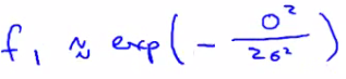
• Which is basically $e^0 = 1$
  • Which is close to 1
• Say x is far from a landmark
  • Then the squared distance is big
    • Gives $e^{-\text{large number}} \approx 0$
      • Which is close to zero
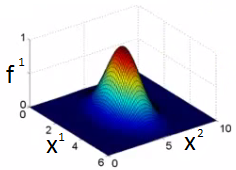
• Each landmark defines a new features
• If we plot f1 vs the kernel function we get a plot like this
  • Notice that when $x = [3, 5]$, then $f_1 = 1$
  • As $x$ moves away from $[3, 5]$, the feature takes on values close to zero
  • So this measures how close x is to this landmark

What Does $\sigma$ Do?

• **$\sigma^2$**is a parameter of the Gaussian kernel
  • Defines the steepness of the rise around the landmark
• Above example $\sigma^2$ = 1
• Below $\sigma^2$ = 0.5

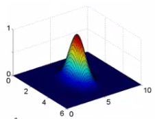
• We see here that as you move away from 3,5 the feature f1 falls to zero much more rapidly
• The inverse can be seen if $\sigma^2$ = 3

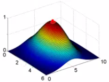
• Given this definition, what kinds of hypotheses can we learn?
  • With training examples x we predict "1" when
  • $\theta_0 + \theta_1 f_1 + \theta_2 f_2 + \theta_3 f_3 \ge 0$
    • For our example, lets say we've already run an algorithm and got the
      • $\theta_0 = -0.5$
      • $\theta_1 = 1$
      • $\theta_2 = 1$
      • $\theta_3 = 0$
    • Given our placement of three examples, what happens if we evaluate an example at the magenta dot below?

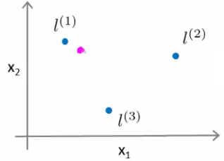
• Looking at our formula, we know $f_1$ will be close to 1, but $f_2$ and $f_3$ will be close to 0
  • So if we look at the formula we have
    • $\theta_0 + \theta_1 f_1 + \theta_2 f_2 + \theta_3 f_3 \ge 0$
    • -0.5 + 1 + 0 + 0 = 0.5
      • 0.5 is greater than 1
• If we had another point far away from all three

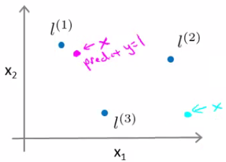
• This equates to -0.5
  • So we predict 0
• Considering our parameters, for points near $l^{(1)}$ and $l^{(2)}$ you predict 1, but for points near $l^{(3)}$ you predict 0
• Which means we create a non-linear decision boundary that goes a lil' something like this;

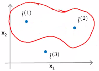
• Inside we predict y = 1
• Outside we predict y = 0
• So this show how we can create a non-linear boundary with landmarks and the kernel function in the support vector machine
• But
• How do we get/chose the landmarks
• What other kernels can we use (other than the Gaussian kernel)

Kernels II

• Filling in missing detail and practical implications regarding kernels
• Spoke about picking landmarks manually, defining the kernel, and building a hypothesis function
  • Where do we get the landmarks from?
  • For complex problems we probably want lots of them

Choosing the Landmarks

• Take the training data
• For each example place a landmark at exactly the same location
• So end up with m landmarks
  • One landmark per location per training example
  • Means our features measure how close to a training set example something is
• Given a new example, compute all the f values
  • Gives you a feature vector f (f_0 to f_m)
    • f_0 = 1 always
• A more detailed look at generating the f vector
  • If we have a training example, features are computed using $(x^{(i)}, y^{(i)})$
    • Cycle through each landmark, calculating how close $x^{(i)}$ is to each landmark:
      • $f_1^{(i)} = k(x^{(i)}, l^{(1)})$
      • $f_2^{(i)} = k(x^{(i)}, l^{(2)})$
      • $\dots$
      • $f_m^{(i)} = k(x^{(i)}, l^{(m)})$
    • Somewhere in the list we compare $x^{(i)}$ to itself (i.e., at feature $f_i^{(i)} = k(x^{(i)}, l^{(i)})$)
      • Since we use the Gaussian Kernel, this evaluates to 1 ($e^0 = 1$)
    • Group these $m$ features $(f_1, f_2, \dots, f_m)$ into an $(m+1) \times 1$ dimensional feature vector $f$:
      • $f^{(i)}$ is the feature vector for the $i$-th example
      • Includes baseline term $f_0^{(i)} = 1$
• Given these kernels, how do we use a support vector machine

SVM hypothesis prediction with kernels

• Predict $y = 1$ if $\theta^T f \ge 0$
  • Because $\theta \in \mathbb{R}^{m+1}$
  • And $f \in \mathbb{R}^{m+1}$
• So, this is how you make a prediction assuming you already have $\theta$
  • How do you get $\theta$?

SVM Training with Kernels

• Use the SVM learning algorithm

• Now, we minimize using f as the feature vector instead of x
• By solving this minimization problem you get the parameters for your SVM
• In this setup, m = n
  • Because number of features is the number of training data examples we have
• One final mathematic detail (not crucial to understand)
  • If we ignore $\theta_0$ then the following is true

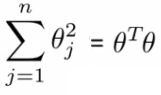
• What many implementations do is

• Where the matrix M depends on the kernel you use

• Gives a slightly different minimization - means we determine a rescaled version of $\theta$

• Allows more efficient computation, and scale to much bigger training sets

• If you have a training set with 10 000 values, means you get 10 000 features

  • Solving for all these parameters can become expensive
  • So by adding this in we avoid a for loop and use a matrix multiplication algorithm instead

• You can apply kernels to other algorithms

  • But they tend to be very computationally expensive
  • But the SVM is far more efficient - so more practical

• Lots of good off the shelf software to minimize this function

• SVM parameters (C)

  • Bias and variance trade off
  • Must chose C
    • C plays a role similar to 1/LAMBDA (where LAMBDA is the regularization parameter)
  • Large C gives a hypothesis of low bias high variance --> overfitting
  • Small C gives a hypothesis of high bias low variance --> underfitting

• SVM parameters ($\sigma^2$)

  • Parameter for calculating f values
    • Large $\sigma^2$ - f features vary more smoothly - higher bias, lower variance
    • Small $\sigma^2$ - f features vary abruptly - low bias, high variance

Support Vector Machines - Implementation and Practical Use

• So far spoken about SVM in a very abstract manner
• What do you need to do this
  • Use SVM software packages (e.g. liblinear, libsvm) to solve parameters $\theta$
  • Need to specify
    • Choice of parameter C
    • Choice of kernel

Choosing a Kernel

• We've looked at the Gaussian kernel
  • Need to define $\sigma$ ($\sigma^2$)
    • Discussed $\sigma^2$
  • When would you chose a Gaussian?
    • If n is small and/or m is large
      • e.g. 2D training set that's large
  • If you're using a Gaussian kernel then you may need to implement the kernel function
    • e.g. a function

fi = kernel(x1,x2)

• Returns a real number
• Some SVM packages will expect you to define kernel
• Although, some SVM implementations include the Gaussian and a few others
  • Gaussian is probably most popular kernel
• NB - make sure you perform feature scaling before using a Gaussian kernel
  • If you don't features with a large value will dominate the f value
• Could use no kernel - linear kernel
  • Predict y = 1 if $\theta^T x$ >= 0
    • So no f vector
    • Get a standard linear classifier
  • Why do this?
    • If n is large and m is small then
      • Lots of features, few examples
      • Not enough data - risk overfitting in a high dimensional feature-space
• Other choice of kernel
  • Linear and Gaussian are most common
  • Not all similarity functions you develop are valid kernels
    • Must satisfy Merecer's Theorem
    • SVM use numerical optimization tricks
      • Mean certain optimizations can be made, but they must follow the theorem
  • Polynomial Kernel
    • We measure the similarity of x and l by doing one of
      • $(x^T l)^2$
      • $(x^T l)^3$
      • $(x^T l + 1)^3$
    • General form is
      • $(x^T l + \text{Const})^D$
    • If they're similar then the inner product tends to be large
    • Not used that often
    • Two parameters
    • Degree of polynomial (D)
    • Number you add to l (Con)
    • Usually performs worse than the Gaussian kernel
    • Used when x and l are both non-negative
  • String kernel
    • Used if input is text strings
    • Use for text classification
  • Chi-squared kernel
  • Histogram intersection kernel

Multi-Class Classification for SVM

• Many packages have built in multi-class classification packages
• Otherwise use one-vs all method
• Not a big issue

Logistic Regression vs. SVM

• When should you use SVM and when is logistic regression more applicable
• If n (features) is large vs. m (training set)
• e.g. text classification problem
• Feature vector dimension is 10 000
• Training set is 10 - 1000
• Then use logistic regression or SVM with a linear kernel
• If n is small and m is intermediate
  • n = 1 - 1000
  • m = 10 - 10 000
  • Gaussian kernel is good
• If n is small and m is large
  • n = 1 - 1000
  • m = 50 000+
    • SVM will be slow to run with Gaussian kernel
  • In that case
    • Manually create or add more features
    • Use logistic regression of SVM with a linear kernel
• Logistic regression and SVM with a linear kernel are pretty similar
  • Do similar things
  • Get similar performance
• A lot of SVM's power is using diferent kernels to learn complex non-linear functions
• For all these regimes a well designed NN should work
  • But, for some of these problems a NN might be slower - SVM well implemented would be faster
• SVM has a convex optimization problem - so you get a global minimum
• It's not always clear how to chose an algorithm
  • Often more important to get enough data
  • Designing new features
  • Debugging the algorithm
• SVM is widely perceived a very powerful learning algorithm