Lecture 06: Logistic Regression
An in-depth explanation of logistic regression for binary and multiclass classification, including hypothesis representation, decision boundaries, cost function formulation, gradient descent, advanced optimization, and the one-vs-all strategy.
Classification
In classification problems, the target variable is a discrete value. We want to develop the logistic regression algorithm to determine which class a new input should fall into.
-
Classification problems:
- Email spam / not spam?
- Online transactions fraudulent (yes / no)?
- Tumor malignant / benign?
-
Target Variable ():
- : Negative class (absence of something, e.g., benign tumor, not spam)
- : Positive class (presence of something, e.g., malignant tumor, spam)
We start with binary class problems, where can take on only two values (0 or 1). Later, we will look at multiclass classification problems, which extend binary classification.
Why Not Use Linear Regression for Classification?
Consider a tumor size vs. malignancy ( or ) dataset. We could try fitting a linear regression model and thresholding its output:
- Predict if
- Predict if
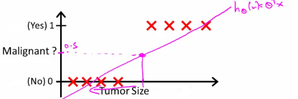
In some simple cases, linear regression with thresholding seems to do a reasonable job of stratifying data points into two classes. However, it suffers from major issues:
- Sensitivity to Outliers: Adding a single positive training example () with a very large tumor size shifts the decision line, causing the threshold to misclassify existing positive examples as negative ().
- Unbounded Hypothesis: We know , but linear regression hypothesis can output values much larger than or less than .
Logistic regression solves this by ensuring hypothesis values always lie strictly between and . Despite the name "regression", logistic regression is a classification algorithm.
Hypothesis Representation
To output values bounded between and , we modify our hypothesis function. In linear regression, we had:
For logistic regression, we wrap inside a function :
Where is defined as:
This function is called the sigmoid function or the logistic function.
Combining these equations gives the logistic regression hypothesis representation:
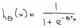
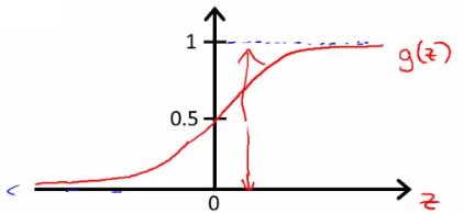
The Sigmoid Function Plot
The sigmoid function crosses at the origin () and asymptotes at (as ) and (as ).
Given this hypothesis representation, our goal is to fit the parameters to our training data.
Interpreting Hypothesis Output
When our hypothesis outputs a number, we interpret that value as the estimated probability that for a given input .
Example
Suppose feature vector contains:
- (bias feature, as always)
If , it tells the patient that they have a probability of the tumor being malignant ().
Formal Probability Notation
This represents: "The probability that , given , parameterized by ."
Since this is a binary classification task where must be either or , the probabilities for the two outcomes must sum to 1:
Decision Boundary
The decision boundary gives a better understanding of what the hypothesis function computes and what its decision regions look like.
To make predictions:
- Predict whenever
- Predict whenever
Looking at the sigmoid curve:
- whenever
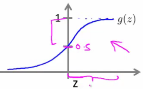
Since :
- whenever
Therefore:
- Hypothesis predicts when
- Hypothesis predicts when
Linear Decision Boundary Example
Consider a system with hypothesis .
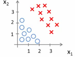
Suppose parameters are chosen as:
The model predicts when:
The line forms the decision boundary.
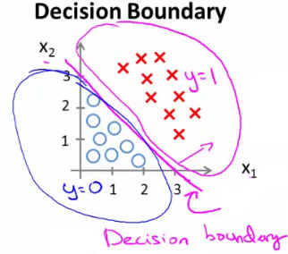
- Magenta ( / ) region: where
- Blue ( / ) region: where
- Straight Line: where exactly.
Key Note: The decision boundary is a property of the hypothesis and its parameters , not of the dataset itself. We fit using dataset training examples, but once is determined, the boundary is defined entirely by .
Non-Linear Decision Boundaries
To fit complex non-linear data distributions, we can add higher-order polynomial features to our input vector, just like in polynomial linear regression.
Suppose our hypothesis includes quadratic terms:
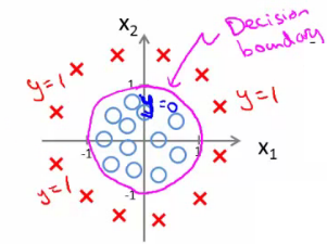
Suppose parameter values are fit as:
The model predicts when:
Plotting yields a circular decision boundary centered at the origin with radius 1:
- Outside the circle (): Predicts
- Inside the circle (): Predicts
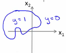
By using even higher-order polynomial features (e.g., ), logistic regression can build arbitrarily complex non-linear decision boundaries (ellipses, complex curves, etc.).
Cost Function for Logistic Regression
Given a training set of examples:
Where each example (with ) and .
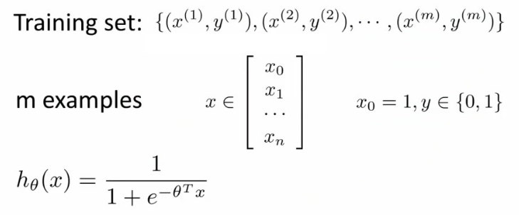
How do we fit the parameters ?
Why Squared Error Fails for Logistic Regression
In linear regression, we used the mean squared error cost function:

If we define the individual example cost as:

Then can be rewritten as:
If we plug the non-linear sigmoid hypothesis into this squared error formula, becomes a non-convex function with many local minima.
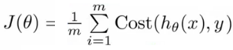
If is non-convex, standard gradient descent is not guaranteed to converge to the global minimum because it can get trapped in local minima.
Convex Logistic Regression Cost Function
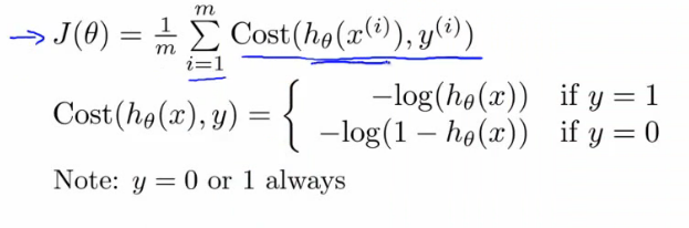
To guarantee global convergence with gradient descent, we need a convex cost function :

Intuition & Plots
- Case :
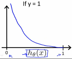
- If and , (perfect prediction, zero penalty).
- As , . This penalizes the model heavily if it predicts probability when .
- Case :
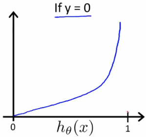
- If and , (perfect prediction, zero penalty).
- As , . This penalizes the model heavily if it predicts probability when .
Using this cost function ensures that is strictly convex and free of local minima.
Simplified Cost Function and Gradient Descent
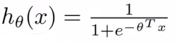
Because in binary classification, we can compress the two cases of into a single line formula:
Verification
- When :
- When :
This compact formulation allows us to express the full cost function as:

Statistical Origin: This cost function is derived from maximum likelihood estimation (MLE) under a Bernoulli likelihood assumption. It is convex and guarantees global optimization.
Gradient Descent Updates
To fit parameters , we want to find that minimizes :
We use gradient descent to iteratively update each parameter :
Calculating the partial derivative of with respect to :
Substituting this back gives the explicit parameter update rule:
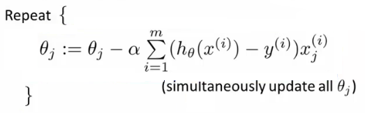
All parameters must be updated simultaneously.
Note: While this parameter update rule looks identical to linear regression, it is NOT identical because for logistic regression is , whereas linear regression uses .
Vectorized Implementation
In vector notation:
Feature scaling (mean normalization, scaling by range/standard deviation) applies to logistic regression gradient descent in the exact same manner as in linear regression to speed up convergence.
Advanced Optimization
For large-scale machine learning problems with many features, standard gradient descent can be slow. Advanced optimization algorithms exist to minimize much faster.
Prerequisites for Optimization Algorithms
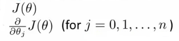
To use optimization routines, we need code that takes as input and computes:
- (the cost value)
- (the partial derivative vector for )
Advanced Optimization Algorithms
- Conjugate Gradient
- BFGS (Broyden-Fletcher-Goldfarb-Shanno)
- L-BFGS (Limited-memory BFGS)
Advantages
- No manual learning rate (): They use an internal line search algorithm to pick optimal step sizes for each iteration.
- Faster convergence: Typically converge much faster than standard gradient descent.
Disadvantages
- More complex; should be accessed via optimized numerical libraries rather than written from scratch.
Using Advanced Optimization Algorithms (Octave / MATLAB)
Consider a simple test optimization problem with two parameters :

1. Define the Cost Function
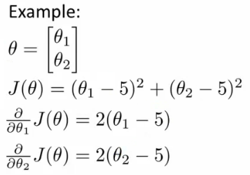
function [jVal, gradient] = costFunction(theta)
  jVal = (theta(1)-5)^2 + (theta(2)-5)^2;
  gradient = zeros(2,1);
  gradient(1) = 2*(theta(1)-5);
  gradient(2) = 2*(theta(2)-5);
end
2. Execute fminunc
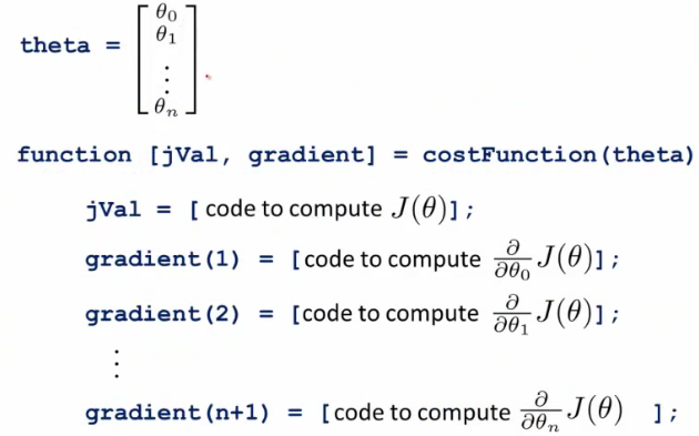
options = optimset('GradObj', 'on', 'MaxIter', 100);
initialTheta = zeros(2,1);

[optTheta, functionVal, exitFlag] = fminunc(@costFunction, initialTheta, options);
optimset('GradObj', 'on', 'MaxIter', 100): Tells Octave thatcostFunctionprovides explicit gradient vectors and sets maximum iterations to 100.fminunc: Stands for find minimum of unconstrained multivariable function.@costFunction: Function handle pointing to the user function.
Multiclass Classification Problems
In multiclass classification, the outcome variable can take on more than two discrete values ().
- Examples:
- Email tagging: Work (), Friends (), Family (), Hobby ()
- Medical diagnosis: Not sick (), Cold (), Flu ()
- Weather: Sunny (), Cloudy (), Rain (), Snow ()
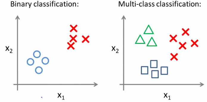
One-vs-All (One-vs-Rest) Classification
The One-vs-All strategy transforms a -class classification problem into separate binary classification problems.
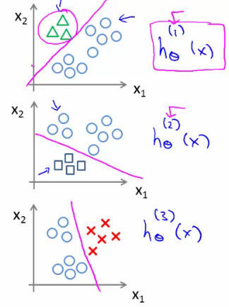
Training Procedure
For a dataset with classes:
- Class 1 vs All: Set class 1 as positive () and all other classes as negative (). Train classifier .
- Class 2 vs All: Set class 2 as positive () and all other classes as negative (). Train classifier .
- Class K vs All: Set class as positive () and all other classes as negative (). Train classifier .
Each classifier evaluates:
Prediction Procedure
Given a new input , evaluate all trained classifiers and pick the class that yields the highest estimated probability:
Lecture 05: Octave
Overview and notes regarding the Octave and MATLAB programming languages used for numerical computation and rapid prototyping in machine learning.
Lecture 07: Regularization
An in-depth guide to regularization in machine learning, covering overfitting, underfitting, regularized cost functions, and regularized linear and logistic regression.