Lecture 14: Dimensionality Reduction

Motivation 1: Data Compression

Dimensionality reduction is a second major class of unsupervised learning problems.

Why Dimensionality Reduction?

• Compression: Reduces the space required to store data on disk or in memory.
• Speedup: Accelerates machine learning algorithms by reducing the number of input features.

What is Dimensionality Reduction?

When building datasets, you may collect a large number of features—sometimes more than necessary. Dimensionality reduction allows us to simplify datasets in a rational and structured way.

Example 1: Redundant Features ($2\text{D} \to 1\text{D}$)

Consider a dataset containing redundant features, such as measuring the same attribute in two different units (e.g., length in centimeters $x_1$ vs. length in inches $x_2$).

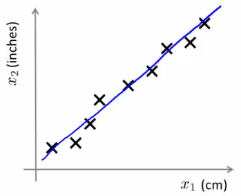
• In real-world data, examples may not lie on a perfect straight line due to measurement noise or round-off errors.
• Data redundancy often occurs when different teams collect data independently without centralized control.
• We can project these 2D points onto a single 1D line to reduce the dataset from 2D to 1D ($2\text{D} \to 1\text{D}$).

Example 2: Pilot Aptitude

In a survey of helicopter pilots:

• $x_1 = \text{pilot skill}$
• $x_2 = \text{pilot enjoyment}$

These features are highly correlated and can be merged into a single summary feature such as "pilot aptitude."

Representing Compressed Data

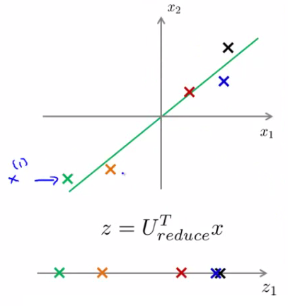
When projecting 2D data onto a line, we record the position of each sample along that single line ($z$):

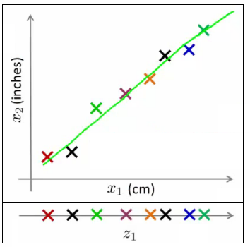
• Original representation: $x^{(1)} \in \mathbb{R}^2$ (a 2D feature vector with $x_1$ and $x_2$ dimensions).
• Compressed representation: $z^{(1)} \in \mathbb{R}^1$ (a single 1D scalar value).
• This cuts storage requirements in half with acceptable lossy compression.

Example 3: $3\text{D} \to 2\text{D}$ Compression

Consider a 3D dataset:

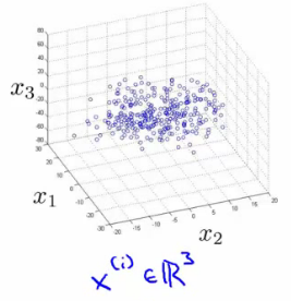
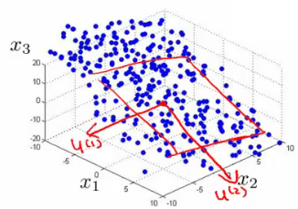
All data points may approximately lie within a 2D plane (e.g., sitting inside a shallow box/tray):

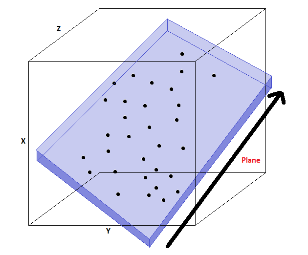
Because the points fall within a shallow depth range, we can drop the perpendicular depth dimension and project the points onto two new axes ($z_1$ and $z_2$) lying on the plane:

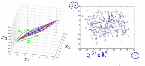
This reduces a 3D feature vector to a 2D feature vector ($3\text{D} \to 2\text{D}$). In large-scale machine learning applications, PCA is often used for massive reductions such as $1000\text{D} \to 100\text{D}$.

Motivation 2: Visualization

It is extremely difficult to visualize data in high dimensions (e.g., 50D). Dimensionality reduction allows us to compress features to 2D or 3D for intuitive visualization and exploration.

Why Visualization Matters

• Understanding data structure helps guide algorithm design.
• Makes it easier to communicate patterns, clusters, and trends to others.

Example: Global Country Statistics

Suppose we collect a dataset containing 50 statistics for various countries:

• $x_1 = \text{GDP}$
• $x_2 = \text{Literacy rate}$
• $\ldots$
• $x_6 = \text{Mean household income}$
• $\ldots, x_{50}$

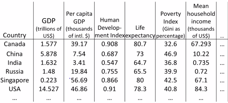
Plotting 50 dimensions directly is impossible. Using dimensionality reduction, we convert each 50-dimensional feature vector $x^{(i)} \in \mathbb{R}^{50}$ into a 2-dimensional vector $z^{(i)} \in \mathbb{R}^2$:

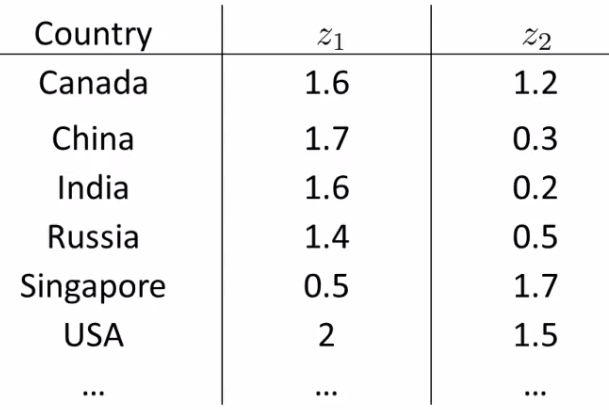
We can then plot the dataset on a 2D graph ($z_1$ vs. $z_2$).

Interpreting Summary Features

Unsupervised learning algorithms do not automatically assign semantic labels to the new dimensions $z_1$ and $z_2$. We inspect the axes to infer their meaning:

• $z_1$ (Horizontal Axis): May correspond to overall country size / total economic output.
• $z_2$ (Vertical Axis): May correspond to per-person well-being or individual economic prosperity.

Feature scaling is crucial prior to dimensionality reduction so all attributes contribute proportionally.

Principal Component Analysis (PCA): Problem Formulation

The most widely used algorithm for dimensionality reduction is Principal Component Analysis (PCA).

Goal of PCA

For $2\text{D} \to 1\text{D}$ reduction, we seek a line onto which the data can be projected:

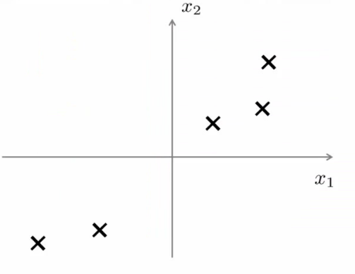
PCA finds a lower-dimensional surface (a line in 2D) that minimizes the projection error (the sum of squared shortest distances from each point to the surface):

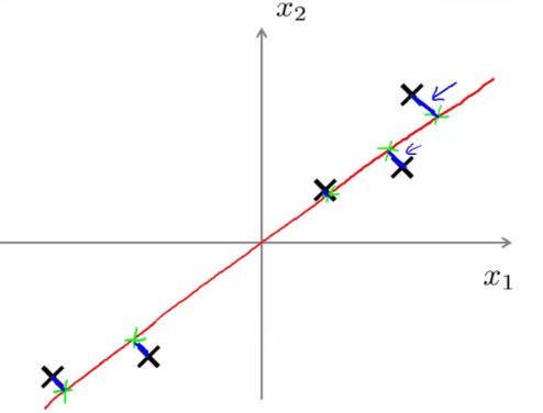
Note: Always perform mean normalization and feature scaling on data before running PCA.

Formal Description

• $2\text{D} \to 1\text{D}$: Find a vector $u^{(1)} \in \mathbb{R}^n$ that defines the projection line minimizing the squared projection error:

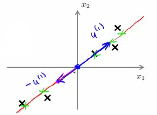
The direction vector $u^{(1)}$ can be positive or negative (i.e., $u^{(1)}$ and $-u^{(1)}$ define the exact same line).

• General Case ($n\text{D} \to k\text{D}$): Find $k$ vectors $u^{(1)}, u^{(2)}, \ldots, u^{(k)} \in \mathbb{R}^n$ onto which to project the data so as to minimize the projection error.
  • The projected points lie on the linear subspace spanned by $\{u^{(1)}, u^{(2)}, \ldots, u^{(k)}\}$.
  • For $3\text{D} \to 2\text{D}$, PCA finds two vectors $u^{(1)}$ and $u^{(2)}$ that define a 2D plane:

PCA vs. Linear Regression

PCA is not linear regression! Despite visual similarities, they minimize entirely different quantities:

• Linear Regression: Minimizes the vertical distance between each point and the fitted line (predicting target $y$ from features $x$).
• PCA: Minimizes the shortest orthogonal (perpendicular) distance between each point and the projection line/surface. All features are treated symmetrically with no separate target label $y$.

PCA Algorithm

1. Data Preprocessing

Given an unlabeled dataset $\{x^{(1)}, x^{(2)}, \ldots, x^{(m)}\}$ where $x^{(i)} \in \mathbb{R}^n$:

1. Mean Normalization:
   • Compute feature means: $\mu_j = \frac{1}{m} \sum_{i=1}^{m} x_j^{(i)}$
   • Replace each $x_j^{(i)}$ with $x_j^{(i)} - \mu_j$ so that every feature has mean $0$.
2. Feature Scaling (if features have different scales):
   • Rescale features: $x_j^{(i)} \leftarrow \frac{x_j^{(i)} - \mu_j}{s_j}$, where $s_j$ is the range ($\text{max} - \text{min}$) or standard deviation.

2. Algorithm Overview ($2\text{D} \to 1\text{D}$)

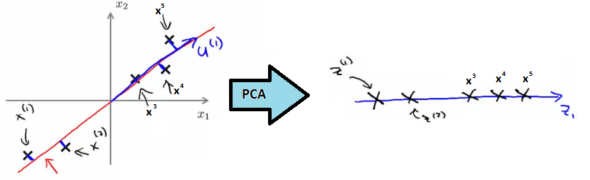
We need to calculate two sets of variables:

1. $u$ vectors: The vectors defining the projection plane/subspace.
2. $z$ vectors: The lower-dimensional feature representations.

3. Step-by-Step Algorithm ($n\text{D} \to k\text{D}$)

Step 1: Compute Covariance Matrix $\Sigma$

$\Sigma = \frac{1}{m} \sum_{i=1}^{m} (x^{(i)})(x^{(i)})^T$

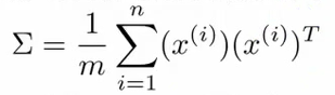
• $\Sigma$ (uppercase Greek letter Sigma) is an $n \times n$ matrix (not to be confused with summation notation).
• $x^{(i)}$ is an $n \times 1$ column vector.

Step 2: Compute Eigenvectors of $\Sigma$

In Octave / MATLAB, compute Singular Value Decomposition (SVD):

[U, S, V] = svd(sigma);

• svd is numerically more stable than eig (eigenvalue decomposition).
• $U$ is an $n \times n$ matrix whose columns are the eigenvectors $u^{(1)}, u^{(2)}, \ldots, u^{(n)}$.
• To reduce from $n\text{D}$ to $k\text{D}$, take the first $k$ columns of $U$:

$U_{\text{reduce}} = \begin{bmatrix} | & | & & | \\ u^{(1)} & u^{(2)} & \dots & u^{(k)} \\ | & | & & | \end{bmatrix} \in \mathbb{R}^{n \times k}$

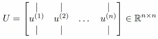
Step 3: Project Data onto Lower Dimension

Calculate $z \in \mathbb{R}^k$ for each example $x \in \mathbb{R}^n$:

$z = U_{\text{reduce}}^T x$

• Dimension check: $U_{\text{reduce}}^T$ is $k \times n$ and $x$ is $n \times 1$, producing $z \in \mathbb{R}^{k \times 1}$.

Summary of PCA Steps

% 1. Preprocess data (mean normalization & scaling)
% 2. Compute covariance matrix
Sigma = (1/m) * (X' * X);

% 3. Compute eigenvectors
[U, S, V] = svd(Sigma);

% 4. Select top k principal components
Ureduce = U(:, 1:k);

% 5. Compute reduced features Z
Z = X * Ureduce; % (m x k)

Reconstruction from Compressed Representation

Since PCA compresses data, can we decompress a low-dimensional vector $z \in \mathbb{R}^k$ back into an approximation of original high-dimensional space $x \in \mathbb{R}^n$?

Reconstruction Formula

Given $z = U_{\text{reduce}}^T x$, the reconstructed feature vector $x_{\text{approx}}$ is:

$x_{\text{approx}} = U_{\text{reduce}} z$

Dimensionality Verification

• $U_{\text{reduce}} \in \mathbb{R}^{n \times k}$
• $z \in \mathbb{R}^{k \times 1}$
• $x_{\text{approx}} = U_{\text{reduce}} z \in \mathbb{R}^{n \times 1}$

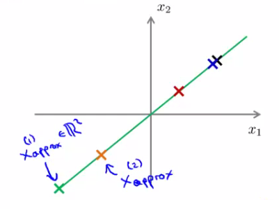
$x_{\text{approx}}$ projects the compressed points back into $n$-dimensional space. While fine detail off the projection line is lost during compression, $x_{\text{approx}}$ closely approximates the original data points.

Choosing the Number of Principal Components

How do we select the parameter $k$ (number of principal components)?

Mathematical Definitions

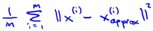
1. Average Squared Projection Error: $\frac{1}{m} \sum_{i=1}^{m} ||x^{(i)} - x_{\text{approx}}^{(i)}||^2$

2. Total Variation in Data: 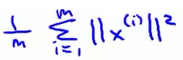$\frac{1}{m} \sum_{i=1}^{m} ||x^{(i)}||^2$ (Average squared distance of training samples from origin).

Variance Retained Ratio

We select $k$ such that the ratio of projection error to total variation is small:

$\frac{\frac{1}{m} \sum_{i=1}^{m} ||x^{(i)} - x_{\text{approx}}^{(i)}||^2}{\frac{1}{m} \sum_{i=1}^{m} ||x^{(i)}||^2} \le 0.01$

When this condition is satisfied, we say that 99% of the variance is retained. Common choices retain 99% or 95% of total variance.

Efficient Selection of $k$

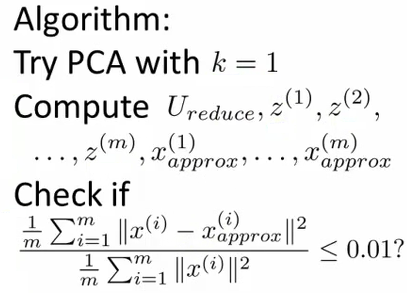
Instead of iteratively running PCA for different values of $k$, use matrix $S$ from a single [U, S, V] = svd(Sigma) call.

$S$ is an $n \times n$ diagonal matrix ($S_{1,1}, S_{2,2}, \ldots, S_{n,n}$). The variance retained ratio simplifies to:

$\frac{\sum_{i=1}^{k} S_{ii}}{\sum_{i=1}^{n} S_{ii}} \ge 0.99$

Test $k = 1, 2, \dots$ until the smallest $k$ satisfying this threshold is found.

Advice for Applying PCA

Speeding Up Supervised Learning Algorithms

Suppose you have a supervised dataset $(x^{(1)}, y^{(1)}), (x^{(2)}, y^{(2)}), \ldots, (x^{(m)}, y^{(m)})$ with very high-dimensional inputs (e.g., $100 \times 100$ image pixels $\implies x \in \mathbb{R}^{10,000}$).

Step-by-Step Implementation

1. Extract features: Form unlabelled set $x^{(1)}, x^{(2)}, \ldots, x^{(m)} \in \mathbb{R}^n$.
2. Run PCA: Map $x^{(i)} \to z^{(i)} \in \mathbb{R}^k$.
3. Form new training set: Pair reduced features with labels $(z^{(1)}, y^{(1)}), \dots, (z^{(m)}, y^{(m)})$.
4. Train model: Train classifier (e.g., logistic regression, neural network) on $(z, y)$.
5. Prediction: For a new test sample $x_{\text{test}}$, apply learned PCA mapping $x_{\text{test}} \to z_{\text{test}}$, then feed $z_{\text{test}}$ to trained model.

CRITICAL RULE: PCA parameters ($\mu, s, U_{\text{reduce}}$) must be learned ONLY on the training set. Once computed, apply these exact parameters to cross-validation and test sets.

PCA typically reduces feature dimensions by $5\times - 10\times$ with minimal impact on predictive performance.

Applications of PCA

Good Applications

1. Compression:
   • Reduces disk/RAM storage.
   • Speeds up learning algorithms.
   • Parameter $k$ chosen based on % variance retained (e.g., 99%).
2. Visualization:
   • Reduces data to $k = 2$ or $k = 3$ for plotting.

Misuse of PCA: Preventing Overfitting

• Flawed Reasoning: Reducing feature count from $n$ to $k$ reduces model capacity and might prevent overfitting.
• Why it fails: PCA discards features without looking at class labels $y$. It may throw away information vital for classification.
• Better Alternative: Use regularization ($\lambda$). Regularization keeps all features while penalizing large weights, producing superior results.

PCA Implementation Advice

• Do not apply PCA prematurely: Start by building and evaluating your machine learning system on raw data without PCA.
• Only add PCA if necessary: Implement PCA only if you observe that training is prohibitively slow or memory usage exceeds system constraints.