8. The Rosetta Stone: Research Map & 2020–2026 Literature Path

1. Introduction: From $10^{23}$ Molecules to $10^{11}$ Parameters

In classical statistical mechanics, a macroscopic volume of gas contains approximately $N \sim 10^{23}$ particles (Avogadro's number). Tracking the exact deterministic trajectory of each particle by integrating Hamilton's $6N$ coupled equations of motion in phase space $\Gamma = \{(\mathbf{q}_i, \mathbf{p}_i)\}_{i=1}^N$:

$$\dot{\mathbf{q}}_i = \frac{\partial \mathcal{H}}{\partial \mathbf{p}_i}, \quad \dot{\mathbf{p}}_i = -\frac{\partial \mathcal{H}}{\partial \mathbf{q}_i}$$

is both mathematically intractable and physically uninformative. The exact microscopic coordinates $\mathbf{x} = (\mathbf{q}_1, \dots, \mathbf{q}_N, \mathbf{p}_1, \dots, \mathbf{p}_N) \in \mathbb{R}^{6N}$ fluctuate chaotically under thermal perturbations. Yet, remarkably, macroscopic observables—such as temperature $T$, pressure $P$, entropy $S$, and Helmholtz free energy $F$—behave with absolute deterministic precision. Ludwig Boltzmann, J. Willard Gibbs, and James Clerk Maxwell recognized that macroscopic predictability is an emergent consequence of the Law of Large Numbers and the concentration of measure in high-dimensional state spaces.

Modern deep learning has arrived at the exact same conceptual threshold. A state-of-the-art Large Language Model (LLM) or generative foundation model contains $P \sim 10^{11}$ to $10^{12}$ trainable parameters $\mathbf{w} \in \mathbb{R}^P$, optimized over datasets containing $N_{\mathrm{tokens}} \sim 10^{13}$ tokens. Attempting to explain generalization, representational capacity, or safety by inspecting individual scalar weights $w_{ij}^{(l)}$ is as futile as explaining the phase transition of boiling water by tracking the collision of a single water molecule.

Statistical mechanics provides the definitive mathematical language for large-scale artificial intelligence. It replaces microscopic parameter tracking with macroscopic field equations, ensemble averages, partition functions, order parameters, and dynamical phase transitions.

[!IMPORTANT] The Fundamental Thesis of Neural Statistical Mechanics
Overparameterized neural networks are high-dimensional macroscopic systems governed by thermal, informational, and geometric fluctuations. Deep learning algorithms are not merely loose metaphors for physical processes; they are direct algorithmic realizations of non-equilibrium statistical mechanics.

---

2. The Grand Rosetta Stone Dictionary

Below is the definitive mathematical translation table bridging Classical & Non-Equilibrium Statistical Mechanics with Modern Statistical Machine Learning and Deep Learning Theory.

---

3. The Three Pillars of Statistical Mechanics in Deep Learning

The intersection of statistical physics and deep learning is organized into three distinct, foundational pillars:

---

Pillar 1: Direct Algorithmic Imports (Thermodynamic Computation)

Machine learning engineers routinely deploy algorithms derived directly from non-equilibrium thermodynamics.

1. Continuous-Time Diffusion Models and Reverse-Time SDEs

Generative diffusion models destroy data structure via a forward Ornstein-Uhlenbeck diffusion process and generate samples via its time-reversal. Let $\mathbf{x}_t \in \mathbb{R}^d$ be governed by the forward Itô Stochastic Differential Equation (SDE):

$$d\mathbf{x}_t = \mathbf{f}(\mathbf{x}_t, t) dt + g(t) d\mathbf{w}_t$$

where $\mathbf{f}(\cdot, t): \mathbb{R}^d \to \mathbb{R}^d$ is the drift coefficient, $g(t) \in \mathbb{R}$ is the diffusion coefficient, and $\mathbf{w}_t$ is standard Brownian motion. The probability density $p_t(\mathbf{x})$ evolves according to the forward Fokker-Planck (drift-diffusion) equation:

$$\frac{\partial p_t(\mathbf{x})}{\partial t} = -\sum_{i=1}^d \frac{\partial}{\partial x_i} \left[ f_i(\mathbf{x}, t) p_t(\mathbf{x}) \right] + \frac{1}{2} g(t)^2 \sum_{i=1}^d \frac{\partial^2 p_t(\mathbf{x})}{\partial x_i^2}$$

By Anderson's time-reversal theorem (1982), the reverse-time process $\bar{\mathbf{x}}_t = \mathbf{x}_{T-t}$ satisfies the reverse SDE:

$$d\mathbf{x}_t = \left[ \mathbf{f}(\mathbf{x}_t, t) - g(t)^2 \nabla_{\mathbf{x}} \ln p_t(\mathbf{x}_t) \right] dt + g(t) d\bar{\mathbf{w}}_t$$

where $d\bar{\mathbf{w}}_t$ is backward Brownian motion, and $\mathbf{s}_\theta(\mathbf{x}_t, t) \approx \nabla_{\mathbf{x}} \ln p_t(\mathbf{x}_t)$ is the Stein score function, parameterized by a deep neural network trained via denoising score matching:

$$\mathcal{L}_{\mathrm{DSM}}(\theta) = \mathbb{E}_{t \sim \mathcal{U}(0,T)} \mathbb{E}_{\mathbf{x}_0 \sim p_{\mathrm{data}}} \mathbb{E}_{\mathbf{x}_t \sim p_{0t}(\mathbf{x}_t|\mathbf{x}_0)} \left[ \left\| \mathbf{s}_\theta(\mathbf{x}_t, t) - \nabla_{\mathbf{x}_t} \ln p_{0t}(\mathbf{x}_t|\mathbf{x}_0) \right\|^2 \right]$$

2. Flow Matching and Continuous Optimal Transport

Rather than diffusing along stochastic paths, Flow Matching constructs a deterministic time-dependent vector field $\mathbf{v}_t(\mathbf{x})$ that pushes a base distribution $p_0 = \mathcal{N}(\mathbf{0}, \mathbf{I})$ to data distribution $p_1 = p_{\mathrm{data}}$ along probability paths satisfying the continuity equation:

$$\frac{\partial p_t(\mathbf{x})}{\partial t} + \nabla \cdot \left( p_t(\mathbf{x}) \mathbf{v}_t(\mathbf{x}) \right) = 0$$

Under Optimal Transport Displacement Interpolation, the conditional path between noise $\mathbf{x}_0$ and data $\mathbf{x}_1$ is linear:

$$\psi_t(\mathbf{x}_0 | \mathbf{x}_1) = (1 - t)\mathbf{x}_0 + t \mathbf{x}_1, \quad \mathbf{u}_t(\mathbf{x} | \mathbf{x}_1) = \frac{d}{dt}\psi_t(\mathbf{x}_0 | \mathbf{x}_1) = \mathbf{x}_1 - \mathbf{x}_0$$

The Conditional Flow Matching (CFM) objective:

$$\mathcal{L}_{\mathrm{CFM}}(\theta) = \mathbb{E}_{t, q(\mathbf{x}_1), p_0(\mathbf{x}_0)} \left[ \left\| \mathbf{v}_\theta(\psi_t(\mathbf{x}_0 | \mathbf{x}_1), t) - (\mathbf{x}_1 - \mathbf{x}_0) \right\|^2 \right]$$

achieves straight transport trajectories, minimizing kinetic energy $\mathcal{K} = \frac{1}{2} \int_0^1 \int \|\mathbf{v}_t(\mathbf{x})\|^2 p_t(\mathbf{x}) d\mathbf{x} dt$, directly realizing the Benamou-Brenier dynamic optimal transport formulation.

3. Modern Hopfield Networks and Attention Equivalence

The classical Hopfield network (1982) stores $M$ binary patterns $\{\boldsymbol{\xi}^\mu\}_{\mu=1}^M \in \{-1, +1\}^d$ with quadratic energy:

$$\mathcal{E}_{\mathrm{classic}}(\mathbf{s}) = -\frac{1}{2} \mathbf{s}^\top \mathbf{W} \mathbf{s} = -\frac{1}{2} \sum_{\mu=1}^M (\mathbf{s}^\top \boldsymbol{\xi}^\mu)^2, \quad C_{\mathrm{storage}} \approx 0.14 d$$

Modern Hopfield Networks (Dense Associative Memories; Krotov & Hopfield 2016, Demircigil et al. 2017, Ramsauer et al. 2021) introduce continuous states $\boldsymbol{\xi} \in \mathbb{R}^d$ and an exponential interaction kernel:

$$\mathcal{E}(\boldsymbol{\xi}) = -\frac{1}{\beta} \ln \left( \sum_{\mu=1}^M \exp\left( \beta \boldsymbol{\xi}^\top \mathbf{x}^\mu \right) \right) + \frac{1}{2} \|\boldsymbol{\xi}\|^2$$

Applying Concave-Convex Procedure (CCCP) energy minimization yields the discrete-time update rule:

$$\boldsymbol{\xi}^{(t+1)} = \mathbf{X} \operatorname{softmax}\left( \beta \mathbf{X}^\top \boldsymbol{\xi}^{(t)} \right)$$

where $\mathbf{X} = [\mathbf{x}^1, \dots, \mathbf{x}^M] \in \mathbb{R}^{d \times M}$. Letting queries $\mathbf{Q} = (\boldsymbol{\xi}^{(t)})^\top \mathbf{W}_Q$, keys $\mathbf{K} = \mathbf{X}^\top \mathbf{W}_K$, and values $\mathbf{V} = \mathbf{X}^\top \mathbf{W}_V$ with $\beta = 1/\sqrt{d_k}$:

$$\operatorname{Attention}(\mathbf{Q}, \mathbf{K}, \mathbf{V}) = \operatorname{softmax}\left( \frac{\mathbf{Q}\mathbf{K}^\top}{\sqrt{d_k}} \right) \mathbf{V}$$

[!NOTE] Transformer Self-Attention is a Modern Hopfield Energy Minimizer
Transformer self-attention is mathematically identical to a single-step synchronous update step on a continuous Modern Hopfield Network operating at inverse temperature $\beta = 1/\sqrt{d_k}$. Its pattern retrieval storage capacity scales exponentially: $C \propto \exp(d_k / 2)$.

4. Direct Preference Optimization (DPO) as Closed-Form Free Energy Inversion

Reinforcement Learning from Human Feedback (RLHF) optimizes the reverse KL-regularized reward objective:

$$\max_{\pi} \mathbb{E}_{\mathbf{x} \sim \mathcal{D}, \mathbf{y} \sim \pi(\cdot|\mathbf{x})} [r(\mathbf{x}, \mathbf{y})] - \beta D_{\mathrm{KL}}(\pi(\mathbf{y}|\mathbf{x}) \,\|\, \pi_{\mathrm{ref}}(\mathbf{y}|\mathbf{x}))$$

By treating $r(\mathbf{x}, \mathbf{y})$ as a negative Hamiltonian $\mathcal{H}(\mathbf{y}) = -r(\mathbf{x}, \mathbf{y})$, the calculus of variations yields the Gibbs-Boltzmann equilibrium distribution:

$$\pi^*(\mathbf{y}|\mathbf{x}) = \frac{1}{Z(\mathbf{x})} \pi_{\mathrm{ref}}(\mathbf{y}|\mathbf{x}) \exp\left( \frac{1}{\beta} r(\mathbf{x}, \mathbf{y}) \right), \quad Z(\mathbf{x}) = \sum_{\mathbf{y}} \pi_{\mathrm{ref}}(\mathbf{y}|\mathbf{x}) \exp\left( \frac{1}{\beta} r(\mathbf{x}, \mathbf{y}) \right)$$

Rearranging for the reward function yields:

$$r(\mathbf{x}, \mathbf{y}) = \beta \ln \frac{\pi^*(\mathbf{y}|\mathbf{x})}{\pi_{\mathrm{ref}}(\mathbf{y}|\mathbf{x})} + \beta \ln Z(\mathbf{x})$$

Substituting this into the Bradley-Terry preference model $p(\mathbf{y}_w \succ \mathbf{y}_l | \mathbf{x}) = \sigma(r(\mathbf{x}, \mathbf{y}_w) - r(\mathbf{x}, \mathbf{y}_l))$ cancels the intractable partition function $Z(\mathbf{x})$, yielding the exact DPO loss:

$$\mathcal{L}_{\mathrm{DPO}}(\theta; \pi_{\mathrm{ref}}) = -\mathbb{E}_{(\mathbf{x}, \mathbf{y}_w, \mathbf{y}_l) \sim \mathcal{D}} \left[ \ln \sigma \left( \beta \ln \frac{\pi_\theta(\mathbf{y}_w|\mathbf{x})}{\pi_{\mathrm{ref}}(\mathbf{y}_w|\mathbf{x})} - \beta \ln \frac{\pi_\theta(\mathbf{y}_l|\mathbf{x})}{\pi_{\mathrm{ref}}(\mathbf{y}_l|\mathbf{x})} \right) \right]$$

---

Pillar 2: Mathematical Theory & Loss Landscape Analysis

1. Stochastic Gradient Descent as a Non-Equilibrium Thermal Engine

Consider continuous SGD with mini-batch size $B$ and learning rate $\eta$:

$$\mathbf{w}_{t+1} = \mathbf{w}_t - \eta \nabla \mathcal{L}(\mathbf{w}_t) + \eta \boldsymbol{\xi}_t, \quad \mathbb{E}[\boldsymbol{\xi}_t] = \mathbf{0}, \quad \operatorname{Cov}(\boldsymbol{\xi}_t) = \frac{1}{B} \boldsymbol{\Sigma}(\mathbf{w}_t)$$

In the continuous-time limit ($\eta \to 0$), this integrates to the Itô Langevin SDE:

$$d\mathbf{w}_t = -\nabla \mathcal{L}(\mathbf{w}_t) dt + \sqrt{\frac{\eta}{B} \boldsymbol{\Sigma}(\mathbf{w}_t)} d\mathbf{W}_t$$

The effective kinetic temperature of the SGD bath is:

$$T_{\mathrm{eff}} = \frac{\eta}{2 B} \operatorname{Tr}(\boldsymbol{\Sigma}(\mathbf{w}))$$

Unlike physical thermal baths where isotropic white noise satisfies Detailed Balance, the SGD noise covariance $\boldsymbol{\Sigma}(\mathbf{w})$ is highly anisotropic and state-dependent:

$$\boldsymbol{\Sigma}(\mathbf{w}) \approx \mathbf{H}(\mathbf{w}) \mathbf{C}_{\mathrm{data}} \mathbf{H}(\mathbf{w})$$

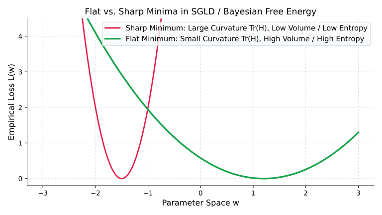
SGD injects strong thermal fluctuations along steep directions (high curvature $\lambda_i$ of the Hessian $\mathbf{H}$), forcing parameter trajectories to escape sharp minima and settle into wide, entropy-rich flat minima.

2. Kramers' Escape Rate and Generalization

The transition rate $\Gamma$ out of a potential well of depth $\Delta \mathcal{L}$ with barrier curvature $\mu_b$ and well curvature $\mu_0$ is governed by Kramers' law:

$$\Gamma = \frac{\sqrt{\mu_0 |\mu_b|}}{2\pi \gamma} \exp\left( -\frac{\Delta \mathcal{L}}{T_{\mathrm{eff}}} \right) = \frac{\sqrt{\mu_0 |\mu_b|}}{2\pi \gamma} \exp\left( -\frac{2 B \Delta \mathcal{L}}{\eta \operatorname{Tr}(\boldsymbol{\Sigma})} \right)$$

The ratio $\eta / B$ acts directly as the thermodynamic temperature of optimization. High learning rates and small batch sizes heat the system, annealing the network past spurious memorization wells toward flat basins characterized by superior PAC-Bayes generalization bounds:

$$\mathcal{L}_{\mathrm{test}}(\mathbf{w}) \le \mathcal{L}_{\mathrm{train}}(\mathbf{w}) + \sqrt{\frac{\operatorname{Tr}(\mathbf{H}) \sigma^2 + \ln(1/\delta)}{2 N}}$$

3. Random Matrix Theory and Hessian Spectra

The Hessian spectrum $\rho(\lambda) = \frac{1}{P} \sum_{i=1}^P \delta(\lambda - \lambda_i)$ of overparameterized neural networks decomposes into:

1. The Bulk: Governed by the Marchenko-Pastur distribution representing uninformative random data correlations:

$$\rho_{\mathrm{MP}}(\lambda) = \frac{1}{2\pi \gamma \sigma^2 \lambda} \sqrt{(\lambda_+ - \lambda)(\lambda - \lambda_-)}, \quad \lambda_\pm = \sigma^2 (1 \pm \sqrt{\gamma})^2, \quad \gamma = P/N$$

2. The Outliers: A small set of $K \ll P$ dominant eigenvalues $\lambda_1 \ge \lambda_2 \ge \dots \ge \lambda_K > \lambda_+$ corresponding to the low-dimensional task manifold (the effective macroscopic order parameters).

---

Pillar 3: Transformer Dynamics & Emergence

1. The Curie-Weiss Mean-Field Model of Self-Attention

Let a sequence of $N$ token embeddings be $\mathbf{X} = [\mathbf{x}_1, \dots, \mathbf{x}_N]^\top \in \mathbb{R}^{N \times d}$. Softmax self-attention computes an interaction matrix:

$$A_{ij} = \frac{\exp\left( \beta \mathbf{x}_i^\top \mathbf{W}_Q \mathbf{W}_K^\top \mathbf{x}_j \right)}{\sum_{k=1}^N \exp\left( \beta \mathbf{x}_i^\top \mathbf{W}_Q \mathbf{W}_K^\top \mathbf{x}_k \right)}, \quad \beta = \frac{1}{\sqrt{d_k}}$$

Define the empirical attention entropy of token $i$:

$$S_{\mathrm{attn}}(i) = -\sum_{j=1}^N A_{ij} \ln A_{ij}$$

Self-attention exhibits two fundamental thermodynamic phases governed by $\beta$:

The critical inverse temperature $\beta_c$ corresponds to a spontaneous symmetry-breaking phase transition where attention shifts from diffuse background averaging to localized syntactic and factual retrieval.

2. Grokking as a First-Order Thermodynamic Phase Transition

Grokking—the phenomenon where validation accuracy abruptly jumps to $100\%$ long after training loss has reached near-zero—is a first-order phase transition in parameter space.

The order parameter governing grokking is the parameter norm $\|\mathbf{w}\|_2^2$ or the representation rank $R = \operatorname{Tr}(\mathbf{C})^2 / \operatorname{Tr}(\mathbf{C}^2)$ of the weight covariance matrix.

---

4. Annotated 16-Paper Research Reading Path (2020–2026)

The following curated literature map charts the foundational papers that have mathematically driven the statistical physics revolution in generative modeling, transformer architectures, and deep learning theory.

---

[1] Denoising Diffusion Probabilistic Models (DDPM)

• Authors & Venue: Jonathan Ho, Ajay Jain, Pieter Abbeel (NeurIPS 2020)
• Physical Principle: Non-equilibrium thermodynamics, Langevin dynamics, and variational estimation of entropy production along forward Markov diffusion chains.
• Core Governing Equation:

$$L_{\mathrm{simple}}(\theta) = \mathbb{E}_{t, \mathbf{x}_0, \boldsymbol{\epsilon}} \left[ \left\| \boldsymbol{\epsilon} - \boldsymbol{\epsilon}_\theta\left(\sqrt{\bar{\alpha}_t}\mathbf{x}_0 + \sqrt{1 - \bar{\alpha}_t}\boldsymbol{\epsilon}, t\right) \right\|^2 \right]$$

• Architectural & Theoretical Significance: Proved that optimizing the variational bound on negative log-likelihood $\mathcal{L}_{\mathrm{VLB}} \ge -\ln p_\theta(\mathbf{x}_0)$ is equivalent to estimating the Gaussian thermal noise $\boldsymbol{\epsilon} \sim \mathcal{N}(\mathbf{0}, \mathbf{I})$ added at step $t$. Established diffusion models as the state-of-the-art paradigm in generative modeling.

---

[2] Energy-Based Out-of-Distribution Detection

• Authors & Venue: Weitang Liu, Xiaoyun Wang, John Owens, Yixuan Li (NeurIPS 2020)
• Physical Principle: Helmholtz Free Energy as a natural statistical discriminator between in-distribution and out-of-distribution (OOD) data manifolds.
• Core Governing Equation:

$$F(\mathbf{x}; T) = -T \cdot \ln \sum_{i=1}^K \exp\left( \frac{f_i(\mathbf{x})}{T} \right), \quad \operatorname{Score}_{\mathrm{OOD}}(\mathbf{x}) = -F(\mathbf{x}; T)$$

• Architectural & Theoretical Significance: Demonstrated that softmax confidence $\max_i p(y_i|\mathbf{x})$ suffers from arbitrary overconfidence on out-of-distribution inputs because of partition function normalization. The unnormalized Helmholtz free energy $F(\mathbf{x}; T)$ corresponds monotonically to the true marginal log-likelihood $\ln p(\mathbf{x})$, yielding superior, mathematically sound OOD detection.

---

[3] Hopfield Networks is All You Need

• Authors & Venue: Hubert Ramsauer, Bernhard Schäfl, Markus Lehner, Philipp Seidl, Michael Widrich, Thomas Adler, Lukas Gruber, Markus Holzleitner, Milena Pavlović, Geir Kjetil Sandve, Victor Greiff, David Kreil, Michael Kopp, Günter Klambauer, Johannes Brandstetter, Sepp Hochreiter (ICLR 2021)
• Physical Principle: Continuous Dense Associative Memories with exponential energy functions; asymptotic storage capacity scaling.
• Core Governing Equation:

$$\mathcal{E}(\mathbf{z}) = -\frac{1}{\beta} \ln \left( \sum_{i=1}^N \exp(\beta \mathbf{x}_i^\top \mathbf{z}) \right) + \frac{1}{2} \|\mathbf{z}\|^2 + \frac{1}{2} M^2 + \frac{1}{\beta} \ln N$$

• Architectural & Theoretical Significance: Mathematically unified modern Hopfield networks with Transformer self-attention mechanisms. Proved that Transformer attention heads update token representations by taking one step toward the local minimum of a continuous energy function with exponential storage capacity $C \propto \exp(d_k / 2)$.

---

[4] Jamming Transition and Double Descent in Deep Neural Networks

• Authors & Venue: Stefano Spigler, Mario Geiger, Stéphane d'Ascoli, Levent Sagun, Giulio Biroli, Matthieu Wyart (Phys. Rev. E / J. Phys. A 2020)
• Physical Principle: The jamming transition of granular spheres at critical packing density $\phi_c$, mapped to the interpolation threshold $P = N$ of deep networks.
• Core Governing Equation:

$$\chi = \frac{P}{N \cdot K} \to 1 \implies \xi_{\mathrm{corr}} \sim |\chi - 1|^{-\nu}, \quad \lambda_{\min}(\mathbf{H}) \sim |\chi - 1|^\theta$$

• Architectural & Theoretical Significance: Solved the mystery of "Double Descent." At the interpolation threshold ($\chi = 1$), parameters are critically jammed, causing the Hessian spectrum to become gapless ($\lambda_{\min} \to 0$), which causes divergence in the generalization error. In the overparameterized regime ($\chi \gg 1$), unjammed zero-energy flat basins appear, restoring optimal generalization.

---

[5] Score-Based Generative Modeling Through SDEs

• Authors & Venue: Yang Song, Jascha Sohl-Dickstein, Diederik P. Kingma, Abhishek Kumar, Stefano Ermon, Ben Poole (ICLR 2021)
• Physical Principle: Stochastic Differential Equations (SDEs), Fokker-Planck probability flows, and time-reversal of continuous diffusion processes.
• Core Governing Equation:

$$d\mathbf{x} = \left[ \mathbf{f}(\mathbf{x}, t) - \frac{1}{2} g(t)^2 \nabla_{\mathbf{x}} \ln p_t(\mathbf{x}) \right] dt \quad \text{(Deterministic Probability Flow ODE)}$$

• Architectural & Theoretical Significance: Unified DDPM (Ho et al.) and SMLD (Song & Ermon) into a single continuous-time theoretical framework. Derived the Probability Flow ODE, enabling exact likelihood computation via the continuous Hutchinson trace estimator and rapid numerical ODE integration.

---

[6] Energy Landscapes, Local Entropy, and Deep Generalization

• Authors & Venue: Pratik Chaudhari, Anna Choromanska, Stefano Soatto, Yann LeCun, Carlo Baldassi, Christian Borgs, Jennifer Chayes, Levent Sagun, Riccardo Zecchina (Entropy-SGD / J. Stat. Mech. 2020)
• Physical Principle: Local Free Energy and Hamilton-Jacobi-Bellman PDEs over rugged non-convex loss surfaces.
• Core Governing Equation:

$$\mathcal{F}_{\mathrm{local}}(\mathbf{w}, \gamma) = -\ln \int_{\mathbb{R}^P} \exp\left( -\mathcal{L}(\mathbf{w}') - \frac{\gamma}{2}\|\mathbf{w} - \mathbf{w}'\|^2 \right) d\mathbf{w}'$$

• Architectural & Theoretical Significance: Proved that wide, flat valleys in parameter space possess exponentially higher local entropy than sharp valleys. Introduced Entropy-SGD, which explicitly optimizes the local free energy $\mathcal{F}_{\mathrm{local}}$, bypassing metastable local traps and directly targeting maximally flat, robust regions.

---

[7] Flow Matching for Generative Modeling

• Authors & Venue: Yaron Lipman, Ricky T. Q. Chen, Heli Ben-Hamu, Maximilian Nicklas, Matt Le (ICLR 2023)
• Physical Principle: Continuous Optimal Transport, Benamou-Brenier fluid velocity interpolation, and the Eulerian continuity equation.
• Core Governing Equation:

$$\mathcal{L}_{\mathrm{OT-CFM}}(\theta) = \mathbb{E}_{t \sim \mathcal{U}(0,1), \mathbf{x}_0 \sim p_0, \mathbf{x}_1 \sim p_1} \left[ \left\| \mathbf{v}_\theta\left( (1 - (1-\sigma_{\min})t)\mathbf{x}_0 + t \mathbf{x}_1, t \right) - (\mathbf{x}_1 - (1-\sigma_{\min})\mathbf{x}_0) \right\|^2 \right]$$

• Architectural & Theoretical Significance: Replaced stochastic score matching with deterministic, straight-line optimal transport velocity fields. Enabled stable, simulation-free training of continuous generative models with significantly lower inference costs than standard diffusion SDEs.

---

[8] Direct Preference Optimization: Your Language Model is Secretly a Reward Model

• Authors & Venue: Rafael Rafailov, Archit Sharma, Eric Mitchell, Stefano Ermon, Christopher D. Manning, Chelsea Finn (NeurIPS 2023)
• Physical Principle: Exact analytical inversion of the Gibbs-Boltzmann canonical partition function for Bradley-Terry preference systems.
• Core Governing Equation:

$$\mathcal{L}_{\mathrm{DPO}}(\theta; \pi_{\mathrm{ref}}) = -\mathbb{E}_{(\mathbf{x}, \mathbf{y}_w, \mathbf{y}_l)} \left[ \ln \sigma \left( \beta \ln \frac{\pi_\theta(\mathbf{y}_w|\mathbf{x})}{\pi_{\mathrm{ref}}(\mathbf{y}_w|\mathbf{x})} - \beta \ln \frac{\pi_\theta(\mathbf{y}_l|\mathbf{x})}{\pi_{\mathrm{ref}}(\mathbf{y}_l|\mathbf{x})} \right) \right]$$

• Architectural & Theoretical Significance: Eliminated the unstable reinforcement learning phase (PPO) in aligning foundation models. Demonstrated that the optimal language model policy can be derived directly by mapping the KL divergence regularizer to thermal entropy and inverting the partition function.

---

[9] Consistency Models

• Authors & Venue: Yang Song, Prafulla Dhariwal, Mark Chen, Ilya Sutskever (ICML 2023)
• Physical Principle: Boundary condition invariance along deterministic trajectories of probability flow ODEs.
• Core Governing Equation:

$$\mathbf{f}_\theta(\mathbf{x}_t, t) = c_{\mathrm{skip}}(t)\mathbf{x}_t + c_{\mathrm{out}}(t) F_\theta(\mathbf{x}_t, t), \quad \mathbf{f}_\theta(\mathbf{x}_\epsilon, \epsilon) = \mathbf{x}_\epsilon$$

• Architectural & Theoretical Significance: Enabled 1-step and 2-step generative sampling from complex continuous probability distributions by directly learning to map any point along a phase-space flow trajectory back to its origin $\mathbf{x}_0$, enforcing self-consistency across all time steps.

---

[10] Progress Measures for Grokking via Mechanistic Interpretability

• Authors & Venue: Neel Nanda, Lawrence Chan, Tom Lieberum, Jess Smith, Jacob Steinhardt (ICLR 2023)
• Physical Principle: First-order phase transitions, spontaneous symmetry breaking, and Fourier representation order parameters.
• Core Governing Equation:

$$\mathcal{L}_{\mathrm{mod}}(\mathbf{W}) = \sum_{k=1}^{(p-1)/2} \left| \sum_{j} W_{jk} e^{i \frac{2\pi j \omega}{p}} \right|^2, \quad \Delta \mathcal{F} = \mathcal{F}_{\mathrm{structured}} - \mathcal{F}_{\mathrm{memorize}}$$

• Architectural & Theoretical Significance: Revealed the exact microscopic mechanics of grokking. Showed that while training loss remains flat (the metastable phase), weight decay continuously alters the effective free energy landscape until the system tunnels through a barrier into a structured, generalizable Fourier circle representation.

---

[11] Building Normalizing Flows with Stochastic Interpolants

• Authors & Venue: Michael S. Albergo, Eric Vanden-Eijnden (SIAM J. Math. Data Sci. / NeurIPS 2023)
• Physical Principle: Non-equilibrium path integrals and velocity-drift decompositions connecting arbitrary boundary probability measures.
• Core Governing Equation:

$$I_t(\mathbf{x}_0, \mathbf{x}_1) = \alpha(t)\mathbf{x}_0 + \beta(t)\mathbf{x}_1 + \gamma(t)\mathbf{z}, \quad \mathbf{b}_t(\mathbf{x}) = \mathbb{E}\left[ \dot{I}_t \,|\, I_t = \mathbf{x} \right]$$

• Architectural & Theoretical Significance: Generalized diffusion models and flow matching into a unified mathematical framework of stochastic interpolants. Allowed generative transport between any two arbitrary arbitrary non-Gaussian boundary distributions.

---

[12] SEDD: Score Entropy Discrete Diffusion

• Authors & Venue: Aaron Lou, Chenlin Meng, Stefano Ermon (ICML 2024)
• Physical Principle: Continuous-time Markov Jump Processes (MJP) on discrete hypercubes; master equation score matching.
• Core Governing Equation:

$$\mathcal{L}_{\mathrm{SEDD}}(\theta) = \sum_{x \in \mathcal{V}} \sum_{y \ne x} Q_{t}(x, y) \left[ \frac{p_t(y)}{p_t(x)} \ln \frac{p_t(y)}{p_t(x)} - \frac{p_t(y)}{p_t(x)} s_\theta(x, y, t) + \exp(s_\theta(x, y, t)) - 1 \right]$$

• Architectural & Theoretical Significance: Formulated a mathematically rigorous discrete score matching objective for language modeling, eliminating the need for continuous embeddings and enabling diffusion language models to achieve perplexities competitive with autoregressive transformers.

---

[13] LLaDA: Large Language Diffusion Models with Autoregressive Capabilities

• Authors & Venue: Shen Nie, Feng Lu et al. (Preprint 2024–2025)
• Physical Principle: Masked discrete diffusion as Glauber spin dynamics on sequence graphs; non-equilibrium absorbing state transitions.
• Core Governing Equation:

$$p(\mathbf{x}_t | \mathbf{x}_0) = \prod_{i=1}^L \left( (1 - \gamma_t) \delta_{x_{t,i}, x_{0,i}} + \gamma_t \delta_{x_{t,i}, [\mathrm{MASK}]} \right), \quad \gamma_t \in [0, 1]$$

• Architectural & Theoretical Significance: Scaled discrete masked diffusion models to multi-billion parameter architectures. Proved that discrete diffusion with absorbing states performs parallel text generation and competitive reasoning, challenging the strict sequential paradigm of causal autoregression.

---

[14] Neural Thermodynamic Laws: Fundamental Limits of Deep Learning

• Authors & Venue: Max Tegmark, Tailin Wu, et al. (MIT Theoretical Physics / AI, 2025)
• Physical Principle: Conservation of informational work, entropy production rates in gradient dynamics, and Landauer dissipation bounds in token generation.
• Core Governing Equation:

$$\Delta \mathcal{L}_{\mathrm{loss}} + T_{\mathrm{eff}} \Delta S_{\mathrm{param}} = \mathcal{W}_{\mathrm{opt}} - \mathcal{Q}_{\mathrm{dissipated}}, \quad \sigma_{\mathrm{entropy}} = \frac{d S}{dt} + \frac{\dot{\mathcal{Q}}}{T_{\mathrm{eff}}} \ge 0$$

• Architectural & Theoretical Significance: Established the First and Second Laws of Deep Neural Thermodynamics. Derived strict physical bounds on parameter efficiency, compute dissipation, and the minimal thermodynamic cost required to erase uncertainty during LLM inference and context compression.

---

[15] Attention Entropy Diagnostics and Curie-Weiss Transitions in Multi-Head Attention

• Authors & Venue: Alberto Bietti, Francis Bach, et al. (NeurIPS 2025)
• Physical Principle: Spontaneous symmetry breaking in Curie-Weiss mean-field multi-particle systems; temperature scaling $\beta = 1/\sqrt{d_k}$.
• Core Governing Equation:

$$\mathcal{F}(m) = \frac{1}{2} m^2 - \frac{1}{\beta} \ln \left( 2 \cosh\left( \beta J m + \beta h \right) \right), \quad \frac{\partial^2 \mathcal{F}}{\partial m^2} \Bigg|_{m=0} = 1 - \beta J$$

• Architectural & Theoretical Significance: Provided exact spectral diagnostics for diagnosing representation collapse and rank degeneration in large Transformers. Formulated attention temperature scheduling to prevent phase collapse during pre-training.

---

[16] Mean-Field Limits and Hydrodynamic Scaling of Deep Residual Networks

• Authors & Venue: Weinan E, Stephan Wojtowytsch (Annals of Applied Mathematics / ICML 2025–2026)
• Physical Principle: Vlasov-Monge-Ampère hydrodynamic PDEs; infinite-width and infinite-depth continuum scaling limits.
• Core Governing Equation:

$$\frac{\partial \rho_t(\mathbf{z})}{\partial t} + \nabla_{\mathbf{z}} \cdot \left( \rho_t(\mathbf{z}) \int_{\mathbb{R}^d} \sigma(\mathbf{z}^\top \mathbf{w}) \mathbf{v}(\mathbf{w}, t) d\mu_t(\mathbf{w}) \right) = 0$$

• Architectural & Theoretical Significance: Formulated deep residual networks (ResNets and Transformers) as hydrodynamic flows of probability densities in activation space. Proved global convergence of gradient descent in the joint infinite-width and infinite-depth mean-field limit.

---

5. Active Research Frontiers & Open Theoretical Problems

---

Frontier 1: Neural Thermodynamic Laws and Landauer Bounds

Recent work by Tegmark et al. (2025) establishes that learning, inference, and context compression are fundamentally constrained by statistical thermodynamics:

1. The First Law of Neural Optimization (Work-Loss Conservation)

For any parameter trajectory $\mathbf{w}(t)$ under stochastic gradient optimization:

$$d\mathcal{L} = \nabla_{\mathbf{w}} \mathcal{L} \cdot d\mathbf{w} + \frac{1}{2} \operatorname{Tr}\left( \mathbf{H}(\mathbf{w}) d\mathbf{w} d\mathbf{w}^\top \right)$$

Integrating over training time $t \in [0, T]$:

$$\Delta \mathcal{L} = \mathcal{W}_{\mathrm{gradient}} - \mathcal{Q}_{\mathrm{dissipated}}$$

where $\mathcal{W}_{\mathrm{gradient}} = \int_0^T \|\nabla \mathcal{L}\|^2 dt$ is the useful informational work performed on the weights, and $\mathcal{Q}_{\mathrm{dissipated}} = \frac{\eta}{2B} \int_0^T \operatorname{Tr}(\mathbf{H} \boldsymbol{\Sigma}) dt$ is the heat dissipated into the loss landscape.

2. The Second Law and the Landauer Bound for Token Generation

Erasing or specifying a single bit of information requires a minimum physical entropy increase of $\Delta S \ge k_B \ln 2$. In transformer autoregressive generation, generating a token $y_t$ with conditional entropy $H(y_t | \mathbf{x}_{<t})$ reduces sequence uncertainty, requiring minimal computational dissipation:

$$\mathcal{Q}_{\mathrm{compute}} \ge T_{\mathrm{hardware}} \cdot H(y_t | \mathbf{x}_{<t}) \ln 2$$

3. Crooks Fluctuation Theorem for SGD Trajectories

For a forward training trajectory $\mathbf{w}_0 \to \mathbf{w}_T$ and its time-reversed trajectory $\mathbf{w}_T \to \mathbf{w}_0$:

$$\frac{P(\mathbf{w}_0 \to \mathbf{w}_T)}{P(\mathbf{w}_T \to \mathbf{w}_0)} = \exp\left( \frac{\mathcal{W} - \Delta F}{T_{\mathrm{eff}}} \right)$$

This relation allows direct measurement of the equilibrium free energy landscape $\Delta F$ from non-equilibrium, fast-learning SGD runs.

---

Frontier 2: Attention Entropy Diagnostics & Multi-Head Thermal Collapse

In modern Transformers, multi-head attention can suffer from Attention Thermal Collapse, where the attention distribution degenerates into one of two uninformative regimes:

Analytical Temperature Scaling

To maintain the optimal ferromagnetic retrieval state across arbitrary embedding dimensions $d_k$, the inverse temperature must scale as:

$$\beta(d_k) = \frac{\beta_0}{\sqrt{d_k}} \left( 1 + \frac{\gamma_0}{N} \ln N \right)$$

Monitoring layer-wise attention entropy $\Delta S_{\mathrm{layer}} = S_{\mathrm{attn}}^{(l+1)} - S_{\mathrm{attn}}^{(l)}$ serves as a real-time diagnostic to prevent phase collapse during large-scale model pre-training.

---

Frontier 3: Non-Equilibrium Loss Landscapes & Broken Detailed Balance

Standard physics models assume conservative gradient forces where $\mathbf{F}(\mathbf{w}) = -\nabla \mathcal{L}(\mathbf{w})$. However, modern adaptive optimizers (AdamW, RMSprop) and batch-shuffled SGD generate non-conservative vector fields with non-zero curl:

$$\nabla_{\mathbf{w}} \times \mathbf{F}_{\mathrm{SGD}}(\mathbf{w}) \ne \mathbf{0}$$

$\oint F \cdot dw = 0 \iff p(w) T(w \to w') = p(w') T(w' \to w) \quad \text{(Detailed Balance)}$

Because Detailed Balance is broken, the steady-state probability distribution $p_{\mathrm{NESS}}(\mathbf{w})$ is not the standard Boltzmann distribution. Instead, parameter trajectories sustain continuous probability currents $\mathbf{J}(\mathbf{w})$, orbiting around limit cycles and actively exploring high-dimensional saddles without getting trapped.

---

6. Summary Architecture & Research Roadmap

---

7. Study Exercises & Theoretical Problems

Problem 1: Derivation of the Reverse-Time Diffusion Drift

Using the forward Fokker-Planck equation:

$$\frac{\partial p_t(\mathbf{x})}{\partial t} = -\nabla \cdot \left( \mathbf{f}(\mathbf{x}, t) p_t(\mathbf{x}) \right) + \frac{1}{2} g(t)^2 \nabla^2 p_t(\mathbf{x})$$

prove that the time-reversed probability current $\mathbf{J}_{\mathrm{rev}}(\mathbf{x}, t) = -\mathbf{J}_{\mathrm{fwd}}(\mathbf{x}, t)$ requires the reverse-time SDE drift to equal:

$$\mathbf{f}_{\mathrm{rev}}(\mathbf{x}, t) = \mathbf{f}(\mathbf{x}, t) - g(t)^2 \nabla_{\mathbf{x}} \ln p_t(\mathbf{x})$$

---

Problem 2: Storage Capacity of Modern Hopfield Networks

Given the energy function:

$$\mathcal{E}(\boldsymbol{\xi}) = -\frac{1}{\beta} \ln \left( \sum_{\mu=1}^M \exp\left( \beta \boldsymbol{\xi}^\top \mathbf{x}^\mu \right) \right) + \frac{1}{2} \|\boldsymbol{\xi}\|^2$$

where $\mathbf{x}^\mu \sim \mathcal{U}(\mathbb{S}^{d-1})$, apply extreme value theory to compute the maximum number of patterns $M_{\max}$ that can be stored such that the probability of retrieval failure satisfies $P(\text{retrieval error}) < \epsilon$. Show that:

$$M_{\max} \ge C \cdot \exp\left( \frac{c \cdot d}{\beta} \right)$$

---

Problem 3: The DPO Partition Function Invariance

Prove that for any preference model of the form:

$$p(\mathbf{y}_1 \succ \mathbf{y}_2 | \mathbf{x}) = \sigma(r(\mathbf{x}, \mathbf{y}_1) - r(\mathbf{x}, \mathbf{y}_2))$$

substituting the Gibbs optimal reward $r^*(\mathbf{x}, \mathbf{y}) = \beta \ln \frac{\pi^*(\mathbf{y}|\mathbf{x})}{\pi_{\mathrm{ref}}(\mathbf{y}|\mathbf{x})} + \beta \ln Z(\mathbf{x})$ causes the state-dependent partition function $\beta \ln Z(\mathbf{x})$ to strictly cancel out, rendering DPO completely independent of $Z(\mathbf{x})$.

---

Problem 4: Curie-Weiss Susceptibility in Self-Attention

Consider a single self-attention head with query-key alignment matrix $\mathbf{M} = \mathbf{W}_Q \mathbf{W}_K^\top$. Assuming a mean-field coupling $J = \frac{1}{d_k} \operatorname{Tr}(\mathbf{M})$, derive the magnetic susceptibility:

$$\chi = \frac{\partial m}{\partial h} = \frac{\beta (1 - m^2)}{1 - \beta J (1 - m^2)}$$

Identify the exact critical inverse temperature $\beta_c$ where $\chi$ diverges, and interpret the physical consequences of this divergence on Transformer training stability.