Free Energy, Variational Inference & Direct Preference Optimization (DPO)

Modern artificial intelligence and statistical physics share a profound foundational principle: the optimal state of any complex system is governed by a fundamental trade-off between energy minimization and entropy maximization.

In classical thermodynamics, this balance is quantified by the Helmholtz Free Energy $F = U - TS$. In Bayesian machine learning, it manifests as the Evidence Lower Bound (ELBO) in Variational Autoencoders (VAEs). In modern large language model (LLM) alignment, it underpins the Reinforcement Learning from Human Feedback (RLHF) objective and explains the breakthrough of Direct Preference Optimization (DPO) (Rafailov et al., 2023).

This chapter presents an end-to-end, mathematically rigorous journey from 19th-century statistical mechanics to state-of-the-art generative model alignment. We demonstrate how the intractable canonical partition function $Z$ that has challenged physicists for over a century is eliminated through pairwise preference modeling.

---

1. Conceptual Rosetta Stone: Physics vs. Deep Learning

Before diving into formal derivations, we establish the exact mapping between statistical mechanics, variational inference, and reinforcement learning / LLM alignment.

---

2. Thermodynamic Potentials and Helmholtz Free Energy

2.1 The Canonical Ensemble and Gibbs-Boltzmann Distribution

Consider a physical system in contact with a large thermal reservoir (heat bath) at constant absolute temperature $T$. The microstates of the system are denoted by $x \in \mathcal{X}$, and each microstate has an associated energy given by the Hamiltonian $E(x) \in \mathbb{R}$.

In the canonical ensemble, the probability of the system occupying microstate $x$ is given by the Gibbs-Boltzmann distribution:

$$p(x) = \frac{1}{Z(\beta)} e^{-\beta E(x)}$$

where $\beta \equiv \frac{1}{k_B T}$ is the inverse temperature (we set Boltzmann's constant $k_B = 1$ throughout this chapter for simplicity, hence $\beta = 1/T$), and $Z(\beta)$ is the canonical partition function:

$$Z(\beta) = \sum_{x \in \mathcal{X}} e^{-\beta E(x)} \quad \text{or} \quad Z(\beta) = \int_{\mathcal{X}} e^{-\beta E(x)} \, dx$$

The partition function acts as the fundamental generating function in statistical mechanics. All macroscopic thermodynamic observables can be derived from derivatives of $\ln Z(\beta)$.

2.2 Thermodynamic Observables from the Partition Function

1. Internal Energy ($U$)

The average or internal energy of the system is the expectation value of the Hamiltonian:

$$\begin{aligned} U \equiv \langle E \rangle &= \sum_{x \in \mathcal{X}} p(x) E(x) \\ &= \sum_{x \in \mathcal{X}} \frac{e^{-\beta E(x)}}{Z(\beta)} E(x) \\ &= -\frac{1}{Z(\beta)} \sum_{x \in \mathcal{X}} \frac{\partial}{\partial \beta} \left( e^{-\beta E(x)} \right) \\ &= -\frac{1}{Z(\beta)} \frac{\partial Z(\beta)}{\partial \beta} \\ &= -\frac{\partial \ln Z(\beta)}{\partial \beta} \end{aligned}$$

2. Heat Capacity and Energy Fluctuations

Differentiating the internal energy with respect to temperature yields the heat capacity at constant volume $C_V$:

$$C_V = \frac{\partial U}{\partial T} = \frac{\partial \beta}{\partial T} \frac{\partial U}{\partial \beta} = \left( -\frac{1}{T^2} \right) \left( -\frac{\partial^2 \ln Z}{\partial \beta^2} \right) = \frac{1}{T^2} \frac{\partial^2 \ln Z}{\partial \beta^2}$$

Evaluating $\frac{\partial^2 \ln Z}{\partial \beta^2}$ directly:

$$\frac{\partial^2 \ln Z}{\partial \beta^2} = -\frac{\partial \langle E \rangle}{\partial \beta} = \langle E^2 \rangle - \langle E \rangle^2 = \operatorname{Var}_p(E)$$

Hence, the variance of energy fluctuations is directly proportional to the heat capacity:

$$\operatorname{Var}_p(E) = T^2 C_V = \frac{1}{\beta^2} C_V$$

3. Gibbs-Shannon Entropy ($S$)

The statistical entropy of the canonical distribution $p(x)$ is:

$$S(p) \equiv -\sum_{x \in \mathcal{X}} p(x) \ln p(x) = -\mathbb{E}_p[\ln p(x)]$$

Substituting the explicit form of $p(x) = \frac{1}{Z} e^{-\beta E(x)}$:

$$\begin{aligned} S(p) &= -\sum_{x \in \mathcal{X}} p(x) \left( -\beta E(x) - \ln Z \right) \\ &= \beta \sum_{x \in \mathcal{X}} p(x) E(x) + \ln Z \sum_{x \in \mathcal{X}} p(x) \\ &= \beta \langle E \rangle + \ln Z \end{aligned}$$

Multiplying by $T = 1/\beta$:

$$T S = \langle E \rangle + T \ln Z$$

2.3 Definition of Helmholtz Free Energy

Rearranging the entropy identity yields the Helmholtz Free Energy $F$:

$$F \equiv U - TS = \langle E \rangle - TS = -T \ln Z = -\frac{1}{\beta} \ln Z$$

---

3. The Variational Free Energy Formulation

In statistical mechanics and probabilistic machine learning alike, we frequently encounter an arbitrary, non-equilibrium trial distribution $q(x)$ that differs from the true equilibrium distribution $p(x)$.

3.1 The Variational Free Energy Functional

For any probability distribution $q(x)$ over the microstate space $\mathcal{X}$, we define the Variational Free Energy functional (also known as Gibbs free energy functional or Helmholtz functional) as:

$$\mathcal{F}[q] \equiv \mathbb{E}_{x \sim q}[E(x)] - T S(q)$$

where:

• $\mathbb{E}_{q}[E(x)] = \sum_x q(x) E(x)$ is the expected energy under trial distribution $q$.
• $S(q) = -\sum_x q(x) \ln q(x) = H(q)$ is the Shannon/Gibbs entropy of $q$.

Expanding this definition:

$$\mathcal{F}[q] = \sum_{x \in \mathcal{X}} q(x) E(x) + T \sum_{x \in \mathcal{X}} q(x) \ln q(x)$$

3.2 Exact Equivalence between Free Energy and KL Divergence

We now prove the central theorem linking statistical mechanics to information theory.

Step-by-Step Proof:

Recall the definition of the Kullback-Leibler (KL) divergence from $q$ to $p$:

$$D_{\mathrm{KL}}(q \,\|\, p) \equiv \sum_{x \in \mathcal{X}} q(x) \ln \frac{q(x)}{p(x)} = \sum_{x \in \mathcal{X}} q(x) \ln q(x) - \sum_{x \in \mathcal{X}} q(x) \ln p(x)$$

Substitute the canonical Gibbs distribution $p(x) = \frac{1}{Z} e^{-\beta E(x)}$ into the second term:

$$\begin{aligned} \ln p(x) &= \ln \left( \frac{1}{Z} e^{-\beta E(x)} \right) \\ &= -\beta E(x) - \ln Z \end{aligned}$$

Now compute $\sum_x q(x) \ln p(x)$:

$$\begin{aligned} \sum_{x \in \mathcal{X}} q(x) \ln p(x) &= \sum_{x \in \mathcal{X}} q(x) \left( -\beta E(x) - \ln Z \right) \\ &= -\beta \sum_{x \in \mathcal{X}} q(x) E(x) - \ln Z \sum_{x \in \mathcal{X}} q(x) \\ &= -\beta \mathbb{E}_q[E(x)] - \ln Z \end{aligned}$$

Substitute this back into the expression for $D_{\mathrm{KL}}(q \,\|\, p)$:

$$\begin{aligned} D_{\mathrm{KL}}(q \,\|\, p) &= \sum_{x \in \mathcal{X}} q(x) \ln q(x) - \left( -\beta \mathbb{E}_q[E(x)] - \ln Z \right) \\ &= -H(q) + \beta \mathbb{E}_q[E(x)] + \ln Z \end{aligned}$$

Multiplying both sides by $T = \frac{1}{\beta}$:

$$T D_{\mathrm{KL}}(q \,\|\, p) = -T H(q) + \mathbb{E}_q[E(x)] + T \ln Z$$

Notice that the first two terms on the right-hand side are precisely the Variational Free Energy $\mathcal{F}[q] = \mathbb{E}_q[E(x)] - T H(q)$:

$$T D_{\mathrm{KL}}(q \,\|\, p) = \mathcal{F}[q] + T \ln Z$$

Rearranging for $\mathcal{F}[q]$:

$$\mathcal{F}[q] = T D_{\mathrm{KL}}(q \,\|\, p) - T \ln Z = T D_{\mathrm{KL}}(q \,\|\, p) + F_{\mathrm{true}}$$

$\blacksquare$

3.3 Corollaries of the Variational Theorem

From this single identity, three profound mathematical and physical conclusions follow immediately:

1. Bogoliubov / Gibbs Free Energy Inequality

Because the KL divergence is strictly non-negative ($D_{\mathrm{KL}}(q \| p) \ge 0$, with equality if and only if $q = p$ almost everywhere):

$$\mathcal{F}[q] \ge -T \ln Z = F_{\mathrm{true}} \quad \forall q$$

The variational free energy $\mathcal{F}[q]$ provides an upper bound on the true equilibrium free energy $F_{\mathrm{true}}$.

2. Exact Equivalence of Optimizers

Since $F_{\mathrm{true}} = -T \ln Z$ does not depend on the trial distribution $q$:

$$\arg\min_q \mathcal{F}[q] = \arg\min_q D_{\mathrm{KL}}(q \,\|\, p)$$

Minimizing the physical variational free energy $\mathcal{F}[q]$ over any parametric family $\mathcal{Q} = \{ q_\theta \}$ is strictly equivalent to minimizing the Kullback-Leibler divergence to the true Boltzmann distribution $p$.

3. Uniqueness of Equilibrium

The global minimum is attained at:

$$q^*(x) = p(x) = \frac{1}{Z} e^{-\beta E(x)}, \quad \text{at which } \mathcal{F}[q^*] = -T \ln Z$$

---

4. Variational Inference & Evidence Lower Bound (ELBO) in Deep Learning

In modern machine learning (e.g., Variational Autoencoders (Kingma & Welling, 2013), latent diffusion models), we observe high-dimensional data $x \sim p_{\mathrm{data}}(x)$ generated by unobserved latent variables $z \in \mathcal{Z}$ through a generative model $p_\theta(x, z) = p(z) p_\theta(x \mid z)$.

4.1 The Intractable Posterior Problem

Computing the true posterior over latents $p_\theta(z \mid x) = \frac{p_\theta(x, z)}{p_\theta(x)}$ requires the marginal likelihood (evidence):

$$p_\theta(x) = \int_{\mathcal{Z}} p_\theta(x, z) \, dz$$

This integral is the exact analog of the continuous partition function $Z(x) = \int e^{-E(x, z)} dz$ where the energy function is the joint negative log-likelihood:

$$E(x, z) \equiv -\ln p_\theta(x, z)$$

For nonlinear deep neural networks, computing $p_\theta(x)$ is computationally intractable due to the curse of dimensionality.

4.2 Derivation of the ELBO from Free Energy

We introduce a variational recognition network $q_\phi(z \mid x)$ to approximate the intractable posterior $p_\theta(z \mid x)$. Setting $T = 1$ ($\beta = 1$), the variational free energy of the posterior approximation is:

$$\mathcal{F}[q_\phi] = \mathbb{E}_{z \sim q_\phi(\cdot|x)} \left[ E(x, z) \right] - H(q_\phi(\cdot \mid x)) = \mathbb{E}_{q_\phi} \left[ -\ln p_\theta(x, z) \right] + \mathbb{E}_{q_\phi} \left[ \ln q_\phi(z \mid x) \right]$$

We define the Evidence Lower Bound (ELBO) as the negative variational free energy:

$$\mathrm{ELBO}(\phi, \theta; x) \equiv -\mathcal{F}[q_\phi]$$

Expanding $\mathrm{ELBO}(\phi, \theta; x)$:

$$\begin{aligned} \mathrm{ELBO}(\phi, \theta; x) &= \mathbb{E}_{z \sim q_\phi(z|x)} \left[ \ln p_\theta(x, z) - \ln q_\phi(z \mid x) \right] \\ &= \mathbb{E}_{z \sim q_\phi(z|x)} \left[ \ln p_\theta(x \mid z) + \ln p(z) - \ln q_\phi(z \mid x) \right] \\ &= \underbrace{\mathbb{E}_{z \sim q_\phi(z|x)} \left[ \ln p_\theta(x \mid z) \right]}_{\text{Reconstruction Fidelity (Negative Energy)}} - \underbrace{D_{\mathrm{KL}}\left( q_\phi(z \mid x) \,\|\, p(z) \right)}_{\text{Prior Regularization (Entropic Penalty)}} \end{aligned}$$

4.3 The Evidence Decomposition

Applying our master free energy identity $\mathcal{F}[q] = D_{\mathrm{KL}}(q \,\|\, p) - \ln Z$ with $Z = p_\theta(x)$:

$$-\mathrm{ELBO}(\phi, \theta; x) = D_{\mathrm{KL}}\left( q_\phi(z \mid x) \,\|\, p_\theta(z \mid x) \right) - \ln p_\theta(x)$$

Rearranging:

$$\ln p_\theta(x) = \mathrm{ELBO}(\phi, \theta; x) + D_{\mathrm{KL}}\left( q_\phi(z \mid x) \,\|\, p_\theta(z \mid x) \right)$$

Since $D_{\mathrm{KL}} \ge 0$, we have $\ln p_\theta(x) \ge \mathrm{ELBO}(\phi, \theta; x)$. Maximizing the ELBO with respect to $\phi$ pushes the variational distribution $q_\phi(z|x)$ toward the true posterior $p_\theta(z|x)$ while simultaneously maximizing the data marginal likelihood $\ln p_\theta(x)$ with respect to generative parameters $\theta$.

---

5. RLHF as Free Energy Minimization

We now transition to language model alignment: training a foundation model $\pi_\theta(y \mid x)$ to produce completions $y \in \mathcal{Y}$ given a prompt $x \in \mathcal{X}$ that align with human preferences.

5.1 The Standard RLHF Objective

In classical Reinforcement Learning from Human Feedback (Ziegler et al., 2019; Ouyang et al., 2022 - InstructGPT), we first train:

1. A Supervised Fine-Tuning (SFT) reference policy $\pi_{\mathrm{ref}}(y \mid x)$.
2. A Reward Model $r_\psi(x, y) \in \mathbb{R}$ parameterized by neural network $\psi$.

We then optimize a parameterized policy $\pi_\theta(y \mid x)$ to maximize expected reward while penalizing divergence from the reference policy $\pi_{\mathrm{ref}}$:

$$\max_{\pi} \mathcal{L}_{\mathrm{RLHF}}(\pi) = \mathbb{E}_{x \sim \mathcal{D}, y \sim \pi(\cdot|x)} \left[ r(x, y) \right] - \beta_{\mathrm{KL}} \, D_{\mathrm{KL}}\left( \pi(\cdot \mid x) \,\|\, \pi_{\mathrm{ref}}(\cdot \mid x) \right)$$

where $\beta_{\mathrm{KL}} > 0$ is the regularization coefficient.

[!WARNING] CRITICAL NOTATION WARNING: $\beta_{\mathrm{KL}}$ in Alignment vs. $\beta$ in Statistical Mechanics In statistical physics:

• $\beta = 1/T$ is the inverse temperature. High $\beta$ means cold / zero exploration.
• $T$ multiplies the entropy term in free energy: $F = \langle E \rangle - T S$.

In machine learning / RLHF literature (Rafailov et al., 2023):

• $\beta_{\mathrm{KL}}$ is the regularization weight multiplying the KL divergence.
• Therefore, $\beta_{\mathrm{KL}}$ plays the mathematical role of Temperature $T$, not inverse temperature!
• Specifically: $T_{\mathrm{effective}} = \beta_{\mathrm{KL}}$, and $\beta_{\mathrm{stat}} = \frac{1}{\beta_{\mathrm{KL}}}$.

As $\beta_{\mathrm{KL}} \to \infty$, the policy is frozen to the prior $\pi_{\mathrm{ref}}$ (infinite temperature / infinite friction). As $\beta_{\mathrm{KL}} \to 0$, the policy collapses onto the greedy reward-maximizing response (zero temperature ground state).

5.2 Deriving the Closed-Form Optimal RLHF Policy

For a fixed prompt $x$, the per-prompt objective to maximize is:

$$J_x(\pi) = \sum_{y \in \mathcal{Y}} \pi(y \mid x) r(x, y) - \beta_{\mathrm{KL}} \sum_{y \in \mathcal{Y}} \pi(y \mid x) \ln \frac{\pi(y \mid x)}{\pi_{\mathrm{ref}}(y \mid x)}$$

subject to the probability normalization constraint $\sum_{y} \pi(y \mid x) = 1$ and $\pi(y \mid x) \ge 0$.

Let us rewrite $-J_x(\pi)$ in the exact form of a Variational Free Energy:

$$\begin{aligned} -J_x(\pi) &= -\sum_{y \in \mathcal{Y}} \pi(y \mid x) r(x, y) + \beta_{\mathrm{KL}} \sum_{y \in \mathcal{Y}} \pi(y \mid x) \ln \pi(y \mid x) - \beta_{\mathrm{KL}} \sum_{y \in \mathcal{Y}} \pi(y \mid x) \ln \pi_{\mathrm{ref}}(y \mid x) \\ &= \sum_{y \in \mathcal{Y}} \pi(y \mid x) \left[ -r(x, y) - \beta_{\mathrm{KL}} \ln \pi_{\mathrm{ref}}(y \mid x) \right] + \beta_{\mathrm{KL}} \sum_{y \in \mathcal{Y}} \pi(y \mid x) \ln \pi(y \mid x) \end{aligned}$$

We define the effective prompt-conditioned Hamiltonian:

$$E(x, y) \equiv -r(x, y) - \beta_{\mathrm{KL}} \ln \pi_{\mathrm{ref}}(y \mid x)$$

Then:

$$-J_x(\pi) = \mathbb{E}_{y \sim \pi(\cdot|x)} \left[ E(x, y) \right] - \beta_{\mathrm{KL}} H(\pi(\cdot \mid x)) = \mathcal{F}[\pi(\cdot \mid x)]$$

with effective temperature $T = \beta_{\mathrm{KL}}$.

By our variational free energy theorem, the distribution $\pi^*(y \mid x)$ that minimizes $\mathcal{F}[\pi]$ (and thus maximizes $J_x(\pi)$) is precisely the canonical Gibbs distribution:

$$\pi^*(y \mid x) = \frac{1}{Z(x)} \exp\left( -\frac{E(x, y)}{\beta_{\mathrm{KL}}} \right)$$

Substitute $E(x, y) = -r(x, y) - \beta_{\mathrm{KL}} \ln \pi_{\mathrm{ref}}(y \mid x)$:

$$\begin{aligned} \pi^*(y \mid x) &= \frac{1}{Z(x)} \exp\left( -\frac{-r(x, y) - \beta_{\mathrm{KL}} \ln \pi_{\mathrm{ref}}(y \mid x)}{\beta_{\mathrm{KL}}} \right) \\ &= \frac{1}{Z(x)} \exp\left( \frac{r(x, y)}{\beta_{\mathrm{KL}}} + \ln \pi_{\mathrm{ref}}(y \mid x) \right) \\ &= \frac{1}{Z(x)} \pi_{\mathrm{ref}}(y \mid x) \exp\left( \frac{r(x, y)}{\beta_{\mathrm{KL}}} \right) \end{aligned}$$

where the per-prompt partition function $Z(x)$ is:

$$Z(x) \equiv \sum_{y \in \mathcal{Y}} \pi_{\mathrm{ref}}(y \mid x) \exp\left( \frac{r(x, y)}{\beta_{\mathrm{KL}}} \right) = \mathbb{E}_{y \sim \pi_{\mathrm{ref}}(\cdot|x)} \left[ \exp\left( \frac{r(x, y)}{\beta_{\mathrm{KL}}} \right) \right]$$

5.3 Alternative Direct Proof via KL Completion

To make this fundamental result unmistakable, we provide a direct algebraic completion of the KL divergence:

$$\begin{aligned} J_x(\pi) &= \sum_{y} \pi(y \mid x) r(x, y) - \beta_{\mathrm{KL}} \sum_y \pi(y \mid x) \ln \frac{\pi(y \mid x)}{\pi_{\mathrm{ref}}(y \mid x)} \\ &= \beta_{\mathrm{KL}} \sum_y \pi(y \mid x) \left[ \frac{r(x, y)}{\beta_{\mathrm{KL}}} - \ln \frac{\pi(y \mid x)}{\pi_{\mathrm{ref}}(y \mid x)} \right] \\ &= \beta_{\mathrm{KL}} \sum_y \pi(y \mid x) \left[ \ln \left( \frac{\pi_{\mathrm{ref}}(y \mid x) \exp(r(x, y)/\beta_{\mathrm{KL}})}{\pi(y \mid x)} \right) \right] \\ &= \beta_{\mathrm{KL}} \sum_y \pi(y \mid x) \left[ \ln \left( \frac{Z(x) \cdot \frac{1}{Z(x)} \pi_{\mathrm{ref}}(y \mid x) \exp(r(x, y)/\beta_{\mathrm{KL}})}{\pi(y \mid x)} \right) \right] \\ &= \beta_{\mathrm{KL}} \sum_y \pi(y \mid x) \ln Z(x) + \beta_{\mathrm{KL}} \sum_y \pi(y \mid x) \ln \left( \frac{\pi^*(y \mid x)}{\pi(y \mid x)} \right) \\ &= \beta_{\mathrm{KL}} \ln Z(x) \underbrace{\sum_y \pi(y \mid x)}_{=1} - \beta_{\mathrm{KL}} \sum_y \pi(y \mid x) \ln \left( \frac{\pi(y \mid x)}{\pi^*(y \mid x)} \right) \\ &= \beta_{\mathrm{KL}} \ln Z(x) - \beta_{\mathrm{KL}} D_{\mathrm{KL}}\left( \pi(\cdot \mid x) \,\|\, \pi^*(\cdot \mid x) \right) \end{aligned}$$

Since $D_{\mathrm{KL}}(\pi \| \pi^*) \ge 0$, the maximum value of $J_x(\pi)$ is achieved if and only if $D_{\mathrm{KL}}(\pi \| \pi^*) = 0$, which uniquely enforces:

$$\pi(y \mid x) = \pi^*(y \mid x) = \frac{1}{Z(x)} \pi_{\mathrm{ref}}(y \mid x) \exp\left( \frac{r(x, y)}{\beta_{\mathrm{KL}}} \right)$$

The corresponding maximum objective value is:

$$J_x(\pi^*) = \beta_{\mathrm{KL}} \ln Z(x) = -F_{\mathrm{eq}}(x)$$

The optimal expected RLHF objective is identically the negative free energy of the aligned language model!

---

6. The Direct Preference Optimization (DPO) Breakthrough

6.1 Why PPO Fails in Practice: The Curse of $Z(x)$

In standard RLHF pipelines, using $\pi^*(y \mid x)$ directly is impossible because:

1. The partition function $Z(x) = \sum_{y \in \mathcal{Y}} \pi_{\mathrm{ref}}(y \mid x) e^{r(x,y)/\beta_{\mathrm{KL}}}$ requires summing over all $|\mathcal{V}|^L$ possible sequences of vocabulary $\mathcal{V}$ and length $L$ (typically $32000^{2048} \approx 10^{9200}$ states).
2. Consequently, traditional pipelines train an approximate reward model $r_\psi(x, y)$, and then run Proximal Policy Optimization (PPO) (Schulman et al., 2017) to optimize $\pi_\theta$.

PPO requires maintaining 4 large models in GPU memory simultaneously:

1. Actor Model $\pi_\theta(y \mid x)$ (active policy)
2. Reference Model $\pi_{\mathrm{ref}}(y \mid x)$ (frozen SFT)
3. Critic / Value Model $V_\phi(x)$ (trained online)
4. Reward Model $r_\psi(x, y)$ (frozen discriminator)

This setup suffers from high variance, unstable gradient updates, high GPU memory footprints, and extreme sensitivity to reward hacking.

6.2 The Bradley-Terry Preference Model

Human preference datasets $\mathcal{D} = \{ (x^{(i)}, y_w^{(i)}, y_l^{(i)}) \}_{i=1}^N$ contain triples where $y_w$ is the winning (preferred) response and $y_l$ is the losing (dispreferred) response for prompt $x$.

Under the Bradley-Terry-Luce (BTL) model of choice (Bradley & Terry, 1952), the probability that a human rater prefers $y_w$ over $y_l$ given an underlying latent ground-truth reward $r^*(x, y)$ is:

$$p^*(y_w \succ y_l \mid x) = \sigma\left( r^*(x, y_w) - r^*(x, y_l) \right) = \frac{1}{1 + \exp\left( -\left( r^*(x, y_w) - r^*(x, y_l) \right) \right)}$$

where $\sigma(u) = \frac{1}{1 + e^{-u}}$ is the standard logistic sigmoid function.

6.3 Inverting the Gibbs Distribution for the Latent Reward

Here comes the ingenious insight of Rafailov et al. (2023): we can analytically invert the optimal policy equation to express the latent reward function $r(x, y)$ purely in terms of the optimal policy $\pi^*(y \mid x)$, the reference policy $\pi_{\mathrm{ref}}(y \mid x)$, and the partition function $Z(x)$.

Take the natural logarithm of both sides of the optimal policy formula:

$$\ln \pi^*(y \mid x) = \ln \pi_{\mathrm{ref}}(y \mid x) + \frac{r^*(x, y)}{\beta_{\mathrm{KL}}} - \ln Z(x)$$

Rearrange for the reward $r^*(x, y)$:

$$\frac{r^*(x, y)}{\beta_{\mathrm{KL}}} = \ln \frac{\pi^*(y \mid x)}{\pi_{\mathrm{ref}}(y \mid x)} + \ln Z(x)$$

Multiplying by $\beta_{\mathrm{KL}}$:

$$r^*(x, y) = \beta_{\mathrm{KL}} \ln \frac{\pi^*(y \mid x)}{\pi_{\mathrm{ref}}(y \mid x)} + \beta_{\mathrm{KL}} \ln Z(x)$$

Notice the two components of the reward:

1. $\beta_{\mathrm{KL}} \ln \frac{\pi^*(y \mid x)}{\pi_{\mathrm{ref}}(y \mid x)}$: The sequence-dependent log-ratio between aligned policy and base policy.
2. $\beta_{\mathrm{KL}} \ln Z(x) = -F_{\mathrm{eq}}(x)$: The free energy baseline, which depends only on the prompt $x$ and is completely independent of the response $y$.

6.4 The Grand Cancellation of the Partition Function

Now, substitute this exact expression for $r^*(x, y)$ into the Bradley-Terry preference probability $p^*(y_w \succ y_l \mid x) = \sigma\left( r^*(x, y_w) - r^*(x, y_l) \right)$:

$$\begin{aligned} r^*(x, y_w) - r^*(x, y_l) &= \left[ \beta_{\mathrm{KL}} \ln \frac{\pi^*(y_w \mid x)}{\pi_{\mathrm{ref}}(y_w \mid x)} + \beta_{\mathrm{KL}} \ln Z(x) \right] - \left[ \beta_{\mathrm{KL}} \ln \frac{\pi^*(y_l \mid x)}{\pi_{\mathrm{ref}}(y_l \mid x)} + \beta_{\mathrm{KL}} \ln Z(x) \right] \\ &= \beta_{\mathrm{KL}} \ln \frac{\pi^*(y_w \mid x)}{\pi_{\mathrm{ref}}(y_w \mid x)} - \beta_{\mathrm{KL}} \ln \frac{\pi^*(y_l \mid x)}{\pi_{\mathrm{ref}}(y_l \mid x)} + \underbrace{\beta_{\mathrm{KL}} \ln Z(x) - \beta_{\mathrm{KL}} \ln Z(x)}_{= 0} \\ &= \beta_{\mathrm{KL}} \ln \left( \frac{\frac{\pi^*(y_w \mid x)}{\pi_{\mathrm{ref}}(y_w \mid x)}}{\frac{\pi^*(y_l \mid x)}{\pi_{\mathrm{ref}}(y_l \mid x)}} \right) \end{aligned}$$

6.5 The DPO Objective Function

We can now directly parameterize $\pi^*(y \mid x)$ with our language model $\pi_\theta(y \mid x)$ and formulate the maximum likelihood objective (binary cross-entropy) on the preference dataset $\mathcal{D}$:

$$\mathcal{L}_{\mathrm{DPO}}(\theta; \pi_{\mathrm{ref}}) = -\mathbb{E}_{(x, y_w, y_l) \sim \mathcal{D}} \left[ \ln \sigma \left( \beta_{\mathrm{KL}} \ln \frac{\pi_\theta(y_w \mid x)}{\pi_{\mathrm{ref}}(y_w \mid x)} - \beta_{\mathrm{KL}} \ln \frac{\pi_\theta(y_l \mid x)}{\pi_{\mathrm{ref}}(y_l \mid x)} \right) \right]$$

We define the implicit reward modeled by the parameterized policy $\pi_\theta$ as:

$$\hat{r}_\theta(x, y) \equiv \beta_{\mathrm{KL}} \ln \frac{\pi_\theta(y \mid x)}{\pi_{\mathrm{ref}}(y \mid x)}$$

Then the DPO loss simplifies cleanly to:

$$\mathcal{L}_{\mathrm{DPO}}(\theta; \pi_{\mathrm{ref}}) = -\mathbb{E}_{(x, y_w, y_l) \sim \mathcal{D}} \left[ \ln \sigma \left( \hat{r}_\theta(x, y_w) - \hat{r}_\theta(x, y_l) \right) \right]$$

---

7. Gradient Analysis & Dynamical Mechanics of DPO

To understand how DPO updates token probabilities during stochastic gradient descent, we compute the exact analytic gradient of $\mathcal{L}_{\mathrm{DPO}}(\theta)$ with respect to network parameters $\theta$.

7.1 Derivation of the DPO Gradient

Let $u \equiv \hat{r}_\theta(x, y_w) - \hat{r}_\theta(x, y_l) = \beta_{\mathrm{KL}} \ln \frac{\pi_\theta(y_w \mid x)}{\pi_{\mathrm{ref}}(y_w \mid x)} - \beta_{\mathrm{KL}} \ln \frac{\pi_\theta(y_l \mid x)}{\pi_{\mathrm{ref}}(y_l \mid x)}$.

Recall the derivative of the log-sigmoid function:

$$\frac{d}{du} \ln \sigma(u) = \frac{1}{\sigma(u)} \cdot \sigma(u)(1 - \sigma(u)) = 1 - \sigma(u) = \sigma(-u)$$

Now apply the chain rule to differentiate $-\ln \sigma(u)$ with respect to $\theta$:

$$\begin{aligned} \nabla_\theta \mathcal{L}_{\mathrm{DPO}}(\theta) &= -\mathbb{E}_{(x, y_w, y_l)} \left[ \sigma\left( -( \hat{r}_\theta(x, y_w) - \hat{r}_\theta(x, y_l) ) \right) \nabla_\theta \left( \hat{r}_\theta(x, y_w) - \hat{r}_\theta(x, y_l) \right) \right] \\ &= -\mathbb{E}_{(x, y_w, y_l)} \left[ \sigma\left( \hat{r}_\theta(x, y_l) - \hat{r}_\theta(x, y_w) \right) \cdot \beta_{\mathrm{KL}} \nabla_\theta \left( \ln \pi_\theta(y_w \mid x) - \ln \pi_\theta(y_l \mid x) \right) \right] \end{aligned}$$

Thus, the DPO gradient is:

$$\nabla_\theta \mathcal{L}_{\mathrm{DPO}}(\theta) = -\beta_{\mathrm{KL}} \, \mathbb{E}_{(x, y_w, y_l) \sim \mathcal{D}} \left[ \underbrace{\sigma\left( \hat{r}_\theta(x, y_l) - \hat{r}_\theta(x, y_w) \right)}_{\text{Implicit Reward Error Weight } w(x, y_w, y_l)} \left( \underbrace{\nabla_\theta \ln \pi_\theta(y_w \mid x)}_{\text{Increase } y_w \text{ probability}} - \underbrace{\nabla_\theta \ln \pi_\theta(y_l \mid x)}_{\text{Decrease } y_l \text{ probability}} \right) \right]$$

7.2 Physical and Algorithmic Interpretation of the Gradient

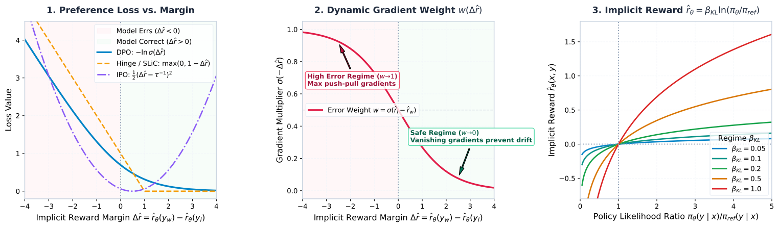
The DPO gradient decomposes into two distinct, intuitive components:

1. Directional Force (Likelihood Push-Pull)

• $\nabla_\theta \ln \pi_\theta(y_w \mid x)$: Increases the log-likelihood of every token in the winning completion $y_w$.
• $-\nabla_\theta \ln \pi_\theta(y_l \mid x)$: Decreases the log-likelihood of every token in the losing completion $y_l$.

2. Adaptive Error Weight $w(x, y_w, y_l) = \sigma(\hat{r}_\theta(x, y_l) - \hat{r}_\theta(x, y_w))$

• High Gradient Regime ($w \to 1$): If the current policy incorrectly rates the losing response higher than the winning response ($\hat{r}_\theta(x, y_l) \gg \hat{r}_\theta(x, y_w)$), then $\hat{r}_\theta(y_l) - \hat{r}_\theta(y_w) \gg 0$, so $\sigma \approx 1$. The model applies the maximum gradient magnitude to correct its mistake.
• Low Gradient Regime ($w \to 0$): If the policy already strongly prefers the winning completion ($\hat{r}_\theta(x, y_w) \gg \hat{r}_\theta(x, y_l)$), then $\sigma \approx 0$, preventing gradient saturation and avoiding catastrophic forgetting.

---

8. Asymptotic Temperature Limits & Phase Transitions

To deepen the statistical mechanics perspective, let us analyze the behavior of the optimal aligned policy $\pi^*(y \mid x)$ under extreme thermodynamic limits of the regularization parameter $\beta_{\mathrm{KL}}$.

8.1 High Temperature Limit ($\beta_{\mathrm{KL}} \to \infty$)

When the regularization parameter is extremely large:

$$\lim_{\beta_{\mathrm{KL}} \to \infty} \frac{r(x, y)}{\beta_{\mathrm{KL}}} = 0 \implies \exp\left( \frac{r(x, y)}{\beta_{\mathrm{KL}}} \right) \to 1$$

The partition function simplifies to:

$$Z(x) \to \sum_{y} \pi_{\mathrm{ref}}(y \mid x) \cdot 1 = 1$$

Thus:

$$\lim_{\beta_{\mathrm{KL}} \to \infty} \pi^*(y \mid x) = \pi_{\mathrm{ref}}(y \mid x)$$

Entropy dominates completely over the energy term. The policy remains identical to the base pre-trained/SFT model.

8.2 Zero Temperature Limit ($\beta_{\mathrm{KL}} \to 0^+$)

When regularization approaches zero, the Boltzmann distribution concentrates all its probability mass on the ground state(s) (i.e., maximum reward completions):

$$\mathcal{Y}^*(x) \equiv \arg\max_{y \in \mathcal{Y}} r(x, y)$$

Let $r_{\max}(x) = \max_y r(x, y)$. Then:

$$\begin{aligned} \pi^*(y \mid x) &= \frac{\pi_{\mathrm{ref}}(y \mid x) e^{(r(x, y) - r_{\max}(x))/\beta_{\mathrm{KL}}}}{\sum_{y'} \pi_{\mathrm{ref}}(y' \mid x) e^{(r(x, y') - r_{\max}(x))/\beta_{\mathrm{KL}}}} \end{aligned}$$

As $\beta_{\mathrm{KL}} \to 0^+$:

• For any $y \notin \mathcal{Y}^*(x)$, $r(x, y) - r_{\max}(x) < 0$, so $e^{(r(x, y) - r_{\max}(x))/\beta_{\mathrm{KL}}} \to 0$.
• For $y \in \mathcal{Y}^*(x)$, $e^0 = 1$.

Therefore:

$$\lim_{\beta_{\mathrm{KL}} \to 0^+} \pi^*(y \mid x) = \begin{cases} \frac{\pi_{\mathrm{ref}}(y \mid x)}{\sum_{y' \in \mathcal{Y}^*(x)} \pi_{\mathrm{ref}}(y' \mid x)} & \text{if } y \in \mathcal{Y}^*(x) \\ 0 & \text{if } y \notin \mathcal{Y}^*(x) \end{cases}$$

If the maximum reward completion $y^*$ is unique, the distribution collapses to a Dirac delta measure:

$$\lim_{\beta_{\mathrm{KL}} \to 0^+} \pi^*(y \mid x) = \delta_{y, y^*}$$

[!CAUTION] Reward Hacking as a Condensation Phase Transition In the zero-temperature regime ($\beta_{\mathrm{KL}} \to 0$), the model experiences a Bose-Einstein-like condensation into the global maximum of the reward model. If the reward model has adversarial vulnerabilities (unnatural repetition, excessive verbosity, sycophancy), the policy collapses into degenerate, ungrammatical gibberish that exploits the proxy reward. Tuning $\beta_{\mathrm{KL}}$ (typically $\beta_{\mathrm{KL}} \in [0.05, 0.5]$) maintains the critical temperature balance between helpful alignment and linguistic entropy.

---

9. Modern Frontiers: Beyond Vanilla DPO (2024–2026)

Following the initial introduction of DPO, the machine learning community discovered subtleties in off-policy preference optimization that led to next-generation algorithms:

9.1 Summary of Frontier Preference Objectives

9.2 The Sequence Length Bias as an Entropic Volume Effect

A well-documented phenomenon in DPO alignment is length bias: models trained with DPO often generate unnecessarily long responses. Statistical mechanics provides an elegant explanation for this behavior:

The log-probability of a sequence $y = (y_1, \dots, y_L)$ is a sum of $L$ token log-probabilities:

$$\ln \pi_\theta(y \mid x) = \sum_{t=1}^L \ln \pi_\theta(y_t \mid x, y_{<t})$$

If the per-token advantage is positive ($\Delta \ln \pi > 0$), longer sequences accumulate a linearly larger total implicit reward $\hat{r}_\theta(x, y) \propto L$. In statistical mechanics, this corresponds to an extensive thermodynamic state variable scaling with system size $V$ (or particle number $N$). Without length normalization (as introduced in SimPO), the system exhibits an entropic expansion toward larger microstate volumes (longer sequences).

---

10. Complete PyTorch Implementation

Below is a production-grade, numerically stable implementation of the DPO loss function, demonstrating how the log-ratio arithmetic and reference policy evaluations are implemented in practice.

"""
Production-Grade Direct Preference Optimization (DPO) Loss Implementation
Includes numerical stability safeguards via logsigmoid and length masking.
"""

import torch
import torch.nn as nn
import torch.nn.functional as F
from typing import Tuple, Optional


class DPOTrainerLoss(nn.Module):
    """
    Direct Preference Optimization (DPO) Loss Module.
    
    Mathematical Formulation:
        L_DPO(theta; pi_ref) = -E_{(x, y_w, y_l)} [ ln sigma( beta * (log_ratio_w - log_ratio_l) ) ]
        where log_ratio = ln pi_theta(y|x) - ln pi_ref(y|x)
    """
    def __init__(
        self, 
        beta: float = 0.1, 
        label_smoothing: float = 0.0,
        length_normalization: bool = False
    ):
        """
        Args:
            beta: Regularization weight (effective temperature T = beta).
            label_smoothing: Conservative label smoothing parameter epsilon.
            length_normalization: Whether to normalize log-probs by sequence length.
        """
        super().__init__()
        self.beta = beta
        self.label_smoothing = label_smoothing
        self.length_normalization = length_normalization

    def _get_batch_logps(
        self,
        logits: torch.FloatTensor,
        labels: torch.LongTensor,
        average_log_prob: bool = False,
        mask_pad_token_id: int = -100
    ) -> torch.FloatTensor:
        """
        Compute sequence-level log-probabilities from model logits.
        
        Args:
            logits: Model forward output logits of shape (batch_size, seq_len, vocab_size).
            labels: Ground-truth target token IDs of shape (batch_size, seq_len).
            average_log_prob: If True, returns mean per-token log-probability.
            mask_pad_token_id: Ignored index for padding tokens.
            
        Returns:
            Per-sequence log-probabilities of shape (batch_size,).
        """
        if logits.shape[:-1] != labels.shape:
            raise ValueError("Logits and labels must have the same batch and sequence dimensions.")

        # Shift logits and labels for autoregressive next-token prediction
        shift_logits = logits[:, :-1, :].contiguous()
        shift_labels = labels[:, 1:].contiguous()
        
        loss_mask = (shift_labels != mask_pad_token_id)
        
        # Log-softmax along vocabulary dimension for numerical precision
        log_probs = F.log_softmax(shift_logits, dim=-1)
        
        # Gather the log-probability of the actual token taken
        # Clamp negative label indices to 0 before gather to prevent index errors
        clamped_labels = shift_labels.clone()
        clamped_labels[~loss_mask] = 0
        
        per_token_logps = torch.gather(
            log_probs, 
            dim=-1, 
            index=clamped_labels.unsqueeze(-1)
        ).squeeze(-1)
        
        # Zero out padding tokens
        per_token_logps = per_token_logps * loss_mask
        
        if average_log_prob:
            seq_lens = loss_mask.sum(dim=-1).clamp(min=1)
            return per_token_logps.sum(dim=-1) / seq_lens
        else:
            return per_token_logps.sum(dim=-1)

    def forward(
        self,
        policy_chosen_logits: torch.FloatTensor,
        policy_rejected_logits: torch.FloatTensor,
        reference_chosen_logits: torch.FloatTensor,
        reference_rejected_logits: torch.FloatTensor,
        chosen_labels: torch.LongTensor,
        rejected_labels: torch.LongTensor,
    ) -> Tuple[torch.FloatTensor, torch.FloatTensor, torch.FloatTensor]:
        """
        Computes the forward pass of DPO loss.
        
        Returns:
            loss: Scalar tensor representing the DPO loss.
            chosen_rewards: Implicit rewards for chosen responses (detached).
            rejected_rewards: Implicit rewards for rejected responses (detached).
        """
        # 1. Compute log-probabilities under the active policy pi_theta
        pi_logps_chosen = self._get_batch_logps(
            policy_chosen_logits, chosen_labels, average_log_prob=self.length_normalization
        )
        pi_logps_rejected = self._get_batch_logps(
            policy_rejected_logits, rejected_labels, average_log_prob=self.length_normalization
        )

        # 2. Compute log-probabilities under the reference policy pi_ref (detached)
        with torch.no_grad():
            ref_logps_chosen = self._get_batch_logps(
                reference_chosen_logits, chosen_labels, average_log_prob=self.length_normalization
            )
            ref_logps_rejected = self._get_batch_logps(
                reference_rejected_logits, rejected_labels, average_log_prob=self.length_normalization
            )

        # 3. Compute log-ratios (log pi_theta - log pi_ref)
        pi_chosen_logratio = pi_logps_chosen - ref_logps_chosen
        pi_rejected_logratio = pi_logps_rejected - ref_logps_rejected

        # 4. Compute implicit rewards: r_hat(x, y) = beta * ln(pi_theta / pi_ref)
        chosen_rewards = self.beta * pi_chosen_logratio.detach()
        rejected_rewards = self.beta * pi_rejected_logratio.detach()

        # 5. Compute preference logits: beta * (logratio_w - logratio_l)
        logits = self.beta * (pi_chosen_logratio - pi_rejected_logratio)

        # 6. Numerically stable loss computation via logsigmoid
        # ln sigma(u) = F.logsigmoid(logits)
        if self.label_smoothing > 0.0:
            # Conservative smoothing: (1 - eps) * BCE + eps * BCE(reversed)
            loss = -(
                (1.0 - self.label_smoothing) * F.logsigmoid(logits)
                + self.label_smoothing * F.logsigmoid(-logits)
            ).mean()
        else:
            loss = -F.logsigmoid(logits).mean()

        return loss, chosen_rewards, rejected_rewards

---

11. Summary of Key Theoretical Insights

---

12. References & Further Reading

1. Boltzmann, L. (1877). Über die Beziehung zwischen dem zweiten Hauptsatze der mechanischen Wärmetheorie und der Wahrscheinlichkeitsrechnung respektive den Sätzen über das Wärmegleichgewicht. Wiener Berichte.
2. Gibbs, J. W. (1902). Elementary Principles in Statistical Mechanics. Yale University Press.
3. Kingma, D. P., & Welling, M. (2013). Auto-Encoding Variational Bayes. arXiv:1312.6114.
4. Ziegler, D. M., et al. (2019). Fine-Tuning Language Models from Human Preferences. arXiv:1909.08593.
5. Ouyang, L., et al. (2022). Training language models to follow instructions with human feedback (InstructGPT). NeurIPS 2022.
6. Rafailov, R., Sharma, A., Mitchell, E., Ermon, S., Manning, C. D., & Finn, C. (2023). Direct Preference Optimization: Your Language Model is Secretly a Reward Model. NeurIPS 2023.
7. Azar, M. G., et al. (2024). A General Theoretical Paradigm to Understand Learning from Human Preferences (IPO). ICML 2024.
8. Ethayarajh, K., et al. (2024). KTO: Model Alignment as Prospect Theoretic Optimization. ICML 2024.
9. Meng, Y., et al. (2024). SimPO: Simple Preference Optimization with a Reference-Free Reward. NeurIPS 2024.
10. Calandriello, D., et al. (2024). Human Alignment of Large Language Models through Online Preference Optimization. ICML 2024.