Spin Glasses, Modern Hopfield Networks & Transformer Attention

In this lecture, we bridge one of the most celebrated domains of modern theoretical physics—the theory of disordered spin systems and spin glasses—with the computational engine driving the deep learning revolution: associative memory architectures and Transformer self-attention.

We will demonstrate that the self-attention mechanism, originally conceived heuristically for sequence transduction, is not merely an engineering trick; it is mathematically identical to a single step of energy minimization in a Continuous Modern Hopfield Network operating in a thermodynamic Gibbs-Boltzmann regime. Furthermore, we explore how the rugged, frustrated free-energy landscapes of spin glasses explain the limits of neural memory, the emergence of hallucinations, the phase transition to In-Context Learning (ICL) in Large Language Models (LLMs), and modern frontiers like Boltzmann Attention.

---

1. The Physics-Deep Learning Rosetta Stone

To establish our conceptual bridge, we begin with a formal translation dictionary between the statistical mechanics of magnetic spin systems and the mathematics of neural associative storage and Transformer architectures.

---

2. From the Ising Model to Disordered Spin Glasses

2.1 The Homogeneous Ising Model

The foundational model of collective magnetic behavior is the Ising Model, defined on a lattice or graph $\mathcal{G} = (\mathcal{V}, \mathcal{E})$ with $N = |\mathcal{V}|$ discrete spins $\sigma_i \in \{-1, +1\}$. The microscopic Hamiltonian is given by:

$$\begin{aligned} H(\boldsymbol{\sigma}) = -J \sum_{\langle i, j \rangle \in \mathcal{E}} \sigma_i \sigma_j - h \sum_{i=1}^N \sigma_i \end{aligned}$$

where:

• $J > 0$ represents a ferromagnetic coupling, which energetically favors parallel alignment ($\sigma_i \sigma_j = +1$).
• $J < 0$ represents an antiferromagnetic coupling, which favors antiparallel alignment ($\sigma_i \sigma_j = -1$).
• $h$ denotes an external magnetic field acting uniformly on all spins.

In thermal equilibrium at temperature $T = 1/\beta$ (setting $k_B = 1$), the probability of finding the system in configuration $\boldsymbol{\sigma}$ is dictated by the canonical Gibbs-Boltzmann distribution:

$$\begin{aligned} P(\boldsymbol{\sigma}) = \frac{1}{Z(\beta, h)} \exp\left( -\beta H(\boldsymbol{\sigma}) \right), \quad Z(\beta, h) = \sum_{\boldsymbol{\sigma} \in \{-1, +1\}^N} \exp\left( -\beta H(\boldsymbol{\sigma}) \right) \end{aligned}$$

The macroscopic order parameter is the average magnetization per spin:

$$\begin{aligned} m = \frac{1}{N} \sum_{i=1}^N \langle \sigma_i \rangle = \frac{1}{N \beta} \frac{\partial \ln Z}{\partial h} \end{aligned}$$

In dimensions $d \ge 2$, the ferromagnetic Ising model exhibits spontaneous symmetry breaking: below a critical Curie temperature $T_c$, the $\mathbb{Z}_2$ spin-flip symmetry ($\boldsymbol{\sigma} \to -\boldsymbol{\sigma}$) is spontaneously broken at $h=0$, yielding two degenerate ground states with non-zero magnetization $m = \pm m_0(T)$.

---

2.2 Quenched Disorder and Frustration

In physical alloys (e.g., dilute magnetic impurities of iron in a gold matrix $\text{Fe}_x \text{Au}_{1-x}$), the atomic positions are fixed on experimental timescales. The exchange interactions fluctuate randomly in sign and magnitude depending on the distance between impurities via the Ruderman-Kittel-Kasuya-Yosida (RKKY) oscillatory interaction:

$$\begin{aligned} J(r) \propto \frac{\cos(2 k_F r)}{r^3} \end{aligned}$$

This introduces two key ingredients defining a spin glass:

1. Quenched Disorder: The couplings $\{J_{ij}\}$ are frozen random variables drawn from a probability distribution $P(J_{ij})$. They do not evolve with the spins on the timescale of microscopic spin flips.
2. Frustration: Geometric or topological impossibility of simultaneously satisfying all pairwise energetic bonds.

Figure 4.1: Frustration in a triangular loop. With two ferromagnetic bonds ($+$) and one antiferromagnetic bond ($-$), setting $\sigma_1 = +1, \sigma_2 = +1$ forces $\sigma_3$ to be $+1$ to satisfy bond $(1,3)$, but $-1$ to satisfy bond $(2,3)$. Both cannot be satisfied simultaneously.

---

2.3 The Sherrington-Kirkpatrick (SK) Model & Mean-Field Spin Glasses

To analyze spin glasses analytically without spatial geometric complications, David Sherrington and Scott Kirkpatrick (1975) introduced the infinite-range mean-field spin glass model.

Quenched vs. Annealed Free Energy

Because the disorder is quenched, the physical free energy per spin is obtained by averaging the logarithm of the partition function over the disorder realizations:

$$\begin{aligned} f = -\frac{1}{\beta N} \mathbb{E}_J \left[ \ln Z(\beta, \{J_{ij}\}) \right] \quad \ne \quad -\frac{1}{\beta N} \ln \mathbb{E}_J \left[ Z(\beta, \{J_{ij}\}) \right] \end{aligned}$$

The calculation of $\mathbb{E}_J[\ln Z]$ requires the Replica Trick:

$$\begin{aligned} \ln Z = \lim_{n \to 0} \frac{Z^n - 1}{n} \implies \mathbb{E}_J[\ln Z] = \lim_{n \to 0} \frac{\mathbb{E}_J[Z^n] - 1}{n} \end{aligned}$$

Evaluating $\mathbb{E}_J[Z^n]$ involves introducing $n$ identical non-interacting replicas of the system, $\{\boldsymbol{\sigma}^a\}_{a=1}^n$, performing the Gaussian integration over $J_{ij}$, and introducing the inter-replica overlap matrix:

$$\begin{aligned} Q_{ab} = \frac{1}{N} \sum_{i=1}^N \sigma_i^a \sigma_i^b \quad (a \ne b) \end{aligned}$$

The Edwards-Anderson Order Parameter & Replica Symmetry Breaking (RSB)

In the spin glass phase ($T < T_{\mathrm{SG}} = J$), the net magnetization vanishes ($m = 0$), but individual spins freeze along arbitrary random local directions ($\langle \sigma_i \rangle \ne 0$). The true order parameter is the Edwards-Anderson order parameter:

$$\begin{aligned} q_{\mathrm{EA}} = \frac{1}{N} \sum_{i=1}^N \langle \sigma_i \rangle^2 \end{aligned}$$

Under Giorgio Parisi’s Full Replica Symmetry Breaking (RSB) solution (Nobel Prize in Physics 2021), the overlap $Q_{ab}$ is not a single number but an entire continuous function $q(x)$ on $x \in [0, 1]$.

Physical Consequences of RSB:

• Rugged Energy Landscape: The free energy surface consists of an exponentially large number $\mathcal{N}_{\mathrm{metastable}} \sim e^{\alpha N}$ of local minima (metastable valleys) separated by divergent free energy barriers in the limit $N \to \infty$.
• Ergodicity Breaking: The phase space breaks into disjoint pure states $\alpha$, with Gibbs decomposition $P(\boldsymbol{\sigma}) = \sum_\alpha w_\alpha P_\alpha(\boldsymbol{\sigma})$.
• Ultrametricity: The overlap distances between any three equilibrium states $\alpha, \beta, \gamma$ satisfy the strong triangle inequality:

$$\begin{aligned} d(\alpha, \gamma) \le \max(d(\alpha, \beta), d(\beta, \gamma)) \end{aligned}$$

---

3. Classical Hopfield Networks and the Limits of Memory

In 1982, John Hopfield recognized that the energy landscape of a disordered Ising system could be engineered to perform content-addressable associative memory. Instead of random couplings $J_{ij}$, the couplings are constructed from a set of $M$ target binary patterns.

3.1 The Model Formulation

Let $\boldsymbol{\xi}^1, \boldsymbol{\xi}^2, \dots, \boldsymbol{\xi}^M \in \{-1, +1\}^N$ be $M$ discrete prototype patterns to be stored. The synaptic weights are determined by the Hebbian Learning Rule:

$$\begin{aligned} J_{ij} = \begin{cases} \displaystyle \frac{1}{N} \sum_{\mu=1}^M \xi_i^\mu \xi_j^\mu & \text{for } i \ne j \\ 0 & \text{for } i = j \end{cases} \end{aligned}$$

In matrix form (with zero diagonal), $J = \frac{1}{N} \sum_{\mu=1}^M \boldsymbol{\xi}^\mu (\boldsymbol{\xi}^\mu)^T - \frac{M}{N} I_N$.

Energy (Lyapunov) Function

The classical Hopfield network is governed by the energy function:

$$\begin{aligned} E(\boldsymbol{\sigma}) = -\frac{1}{2} \sum_{i \ne j} J_{ij} \sigma_i \sigma_j = -\frac{1}{2N} \sum_{\mu=1}^M \left( \sum_{i=1}^N \xi_i^\mu \sigma_i \right)^2 + \frac{M}{2} \end{aligned}$$

Writing the overlap (magnetization) with pattern $\mu$ as:

$$\begin{aligned} m^\mu(\boldsymbol{\sigma}) = \frac{1}{N} \boldsymbol{\xi}^{\mu T} \boldsymbol{\sigma} = \frac{1}{N} \sum_{i=1}^N \xi_i^\mu \sigma_i \in [-1, 1] \end{aligned}$$

The energy is expressed purely in terms of macroscopic overlaps:

$$\begin{aligned} E(\boldsymbol{\sigma}) = -\frac{N}{2} \sum_{\mu=1}^M (m^\mu(\boldsymbol{\sigma}))^2 + \text{const} \end{aligned}$$

Dynamical Update Rule

Under asynchronous Glauber dynamics at $T=0$, a single spin $i$ is updated according to its local alignment field $h_i$:

$$\begin{aligned} h_i = \sum_{j=1}^N J_{ij} \sigma_j, \quad \sigma_i^{(t+1)} = \operatorname{sgn}(h_i) = \operatorname{sgn}\left( \sum_{j \ne i} J_{ij} \sigma_j^{(t)} \right) \end{aligned}$$

---

3.2 The Amit-Gutfreund-Sompolinsky (AGS) Theory of Storage Capacity

What is the maximum number of patterns $M_{\max}$ that can be stored before retrieval catastrophically collapses? This was solved by Daniel Amit, Hanoch Gutfreund, and Haim Sompolinsky (AGS, 1985) using replica theory for the load parameter $\alpha = M/N$.

Signal-to-Noise Analysis

Suppose the network is initialized in the vicinity of target pattern $\boldsymbol{\xi}^1$ ($\boldsymbol{\sigma} \approx \boldsymbol{\xi}^1$). The local field acting on spin $i$ is:

$$\begin{aligned} h_i &= \sum_{j \ne i} \left( \frac{1}{N} \sum_{\mu=1}^M \xi_i^\mu \xi_j^\mu \right) \sigma_j \\ &= \xi_i^1 \left( \frac{1}{N} \sum_{j \ne i} \xi_j^1 \sigma_j \right) + \sum_{\mu=2}^M \xi_i^\mu \left( \frac{1}{N} \sum_{j \ne i} \xi_j^\mu \sigma_j \right) \\ &= \underbrace{\xi_i^1 m^1}_{\text{Signal Term}} + \underbrace{\frac{1}{N} \sum_{\mu=2}^M \sum_{j \ne i} \xi_i^\mu \xi_j^\mu \sigma_j}_{\text{Crosstalk Noise Term } \eta_i} \end{aligned}$$

Assuming random independent patterns $\mathbb{P}(\xi_i^\mu = \pm 1) = 1/2$, the noise term $\eta_i$ is a sum of $(M-1)(N-1) \approx M N$ zero-mean random variables. By the Central Limit Theorem:

$$\begin{aligned} \mathbb{E}[\eta_i] = 0, \quad \operatorname{Var}(\eta_i) = \frac{1}{N^2} \sum_{\mu=2}^M \sum_{j \ne i} (\xi_i^\mu \xi_j^\mu \sigma_j)^2 \approx \frac{M N}{N^2} = \frac{M}{N} = \alpha \end{aligned}$$

Thus, $\eta_i \sim \mathcal{N}(0, \alpha)$. The probability of a bit retrieval error on spin $i$ is:

$$\begin{aligned} P_{\mathrm{error}} = \mathbb{P}(\operatorname{sgn}(h_i) \ne \xi_i^1) = \mathbb{P}(\eta_i < -m^1) = \Phi\left( -\frac{m^1}{\sqrt{\alpha}} \right) = \frac{1}{2} \operatorname{erfc}\left( \frac{m^1}{\sqrt{2\alpha}} \right) \end{aligned}$$

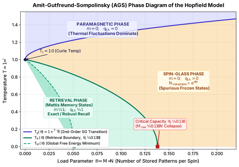Figure 4.2: The AGS Phase Diagram. Below $\alpha_c \approx 0.138$, deep Mattis memory basins exist. Beyond $\alpha_c$, the network undergoes a first-order phase transition into a frozen spin-glass state dominated by spurious minima.

The AGS Phase Regimes:

1. Retrieval Phase ($\alpha < \alpha_c \approx 0.138$): The stored patterns are stable local minima (Mattis states $m^1 \approx 0.97$ at $\alpha_c$).
2. Spin-Glass Phase ($\alpha_c < \alpha < \alpha_{\mathrm{SG}} \approx 0.14$): Retrieval states become metastable and destabilize; the landscape is dominated by exponentially many disordered spin-glass attractors ($m=0, q_{\mathrm{EA}} > 0$).
3. Paramagnetic Phase ($T > T_c(\alpha)$): Thermal fluctuations destroy all magnetic and glass ordering ($m=0, q_{\mathrm{EA}} = 0$).

---

4. Dense Associative Memories & Continuous Modern Hopfield Networks

To overcome the linear capacity limit, Krotov and Hopfield (2016) and Demircigil et al. (2017) revolutionized associative memory by introducing non-polynomial interaction energies.

4.1 Dense Associative Memories (DAM)

Consider an energy function defined by an arbitrary nonlinear interaction potential $F(u)$:

$$\begin{aligned} E(\boldsymbol{\sigma}) = -\sum_{\mu=1}^M F\left( \frac{1}{N} \boldsymbol{\xi}^{\mu T} \boldsymbol{\sigma} \right) \end{aligned}$$

• For $F(u) = \frac{1}{2} u^2$, this reproduces the classical pairwise Hopfield network ($M_{\max} \propto N$).
• For polynomial interactions $F(u) = u^n$ ($n \ge 3$), the interactions become $n$-spin tensor interactions:

$$\begin{aligned} E_n(\boldsymbol{\sigma}) = -\frac{1}{N^{n-1}} \sum_{\mu=1}^M \sum_{i_1, i_2, \dots, i_n} \xi_{i_1}^\mu \xi_{i_2}^\mu \dots \xi_{i_n}^\mu \sigma_{i_1} \sigma_{i_2} \dots \sigma_{i_n} \end{aligned}$$

The storage capacity scales as $M_{\max} \propto N^{n-1}$.

• When $F(u) = \exp(u)$, Demircigil et al. (2017) proved that the storage capacity becomes exponential in dimension:

$$\begin{aligned} M_{\max} \propto 2^{N/2} \quad \text{or} \quad \mathcal{O}(e^{\alpha N}) \end{aligned}$$

---

4.2 Continuous Modern Hopfield Networks (Ramsauer et al., ICLR 2021)

Hubert Ramsauer, Bernhard Schäfl, and Sepp Hochreiter generalized exponential dense associative memories to continuous state vectors $\mathbf{z} \in \mathbb{R}^d$.

4.3 Derivation of the Update Rule via the Concave-Convex Procedure (CCCP)

We now derive the discrete-time update rule for minimizing $E(\mathbf{z})$. Notice that $E(\mathbf{z})$ can be split into a convex term and a concave term:

$$\begin{aligned} E(\mathbf{z}) = \underbrace{\frac{1}{2} \|\mathbf{z}\|^2}_{E_{\mathrm{convex}}(\mathbf{z})} - \underbrace{\beta^{-1} \ln\left( \sum_{\mu=1}^M \exp(\beta \mathbf{x}_\mu^T \mathbf{z}) \right)}_{E_{\mathrm{concave}}(\mathbf{z})} + \text{const} \end{aligned}$$

Using the Concave-Convex Procedure (Yuille & Rangarajan, 2003), we minimize $E(\mathbf{z})$ iteratively by setting the gradient of the convex part at step $t+1$ equal to the negative gradient of the concave part at step $t$:

$$\begin{aligned} \nabla_{\mathbf{z}} E_{\mathrm{convex}}(\mathbf{z}^{(t+1)}) = \nabla_{\mathbf{z}} E_{\mathrm{concave}}(\mathbf{z}^{(t)}) \end{aligned}$$

Let us compute both gradients explicitly:

1. Convex gradient:

$$\begin{aligned} \nabla_{\mathbf{z}} E_{\mathrm{convex}}(\mathbf{z}^{(t+1)}) = \nabla_{\mathbf{z}} \left( \frac{1}{2} \|\mathbf{z}^{(t+1)}\|^2 \right) = \mathbf{z}^{(t+1)} \end{aligned}$$

2. Concave gradient:

$$\begin{aligned} \nabla_{\mathbf{z}} E_{\mathrm{concave}}(\mathbf{z}^{(t)}) &= \nabla_{\mathbf{z}} \left[ \beta^{-1} \ln\left( \sum_{\mu=1}^M \exp(\beta \mathbf{x}_\mu^T \mathbf{z}^{(t)}) \right) \right] \\ &= \beta^{-1} \frac{\sum_{\mu=1}^M \exp(\beta \mathbf{x}_\mu^T \mathbf{z}^{(t)}) \cdot \beta \mathbf{x}_\mu}{\sum_{\nu=1}^M \exp(\beta \mathbf{x}_\nu^T \mathbf{z}^{(t)})} \\ &= \sum_{\mu=1}^M \left( \frac{\exp(\beta \mathbf{x}_\mu^T \mathbf{z}^{(t)})}{\sum_{\nu=1}^M \exp(\beta \mathbf{x}_\nu^T \mathbf{z}^{(t)})} \right) \mathbf{x}_\mu \\ &= X \operatorname{softmax}\left( \beta X^T \mathbf{z}^{(t)} \right) \end{aligned}$$

Equating the two yields the Modern Continuous Hopfield Update Rule:

$$\begin{aligned} \mathbf{z}^{(t+1)} = X \operatorname{softmax}\left( \beta X^T \mathbf{z}^{(t)} \right) \end{aligned}$$

---

4.4 Exponential Storage Capacity in Continuous Spaces

---

5. The Exact Equivalence: Modern Hopfield Networks and Transformer Self-Attention

We now arrive at the central unifying insight: the ubiquitous Transformer Self-Attention mechanism (Vaswani et al., 2017) is mathematically identical to a single-step recall operation in a continuous Modern Hopfield Network.

5.1 Step-by-Step Mathematical Identification

Let us write the standard scaled dot-product attention for a single query vector $\mathbf{q} \in \mathbb{R}^{d_k}$, a key matrix $K = [\mathbf{k}_1, \dots, \mathbf{k}_M]^T \in \mathbb{R}^{M \times d_k}$, and a value matrix $V = [\mathbf{v}_1, \dots, \mathbf{v}_M]^T \in \mathbb{R}^{M \times d_v}$:

$$\begin{aligned} \operatorname{Attn}(\mathbf{q}, K, V) = \operatorname{softmax}\left( \frac{\mathbf{q} K^T}{\sqrt{d_k}} \right) V \end{aligned}$$

Let us expand this row vector formulation into standard column vector notation:

$$\begin{aligned} \mathbf{z}_{\mathrm{out}} = \operatorname{Attn}(\mathbf{q}, K, V)^T = V^T \operatorname{softmax}\left( \frac{K \mathbf{q}}{\sqrt{d_k}} \right) = \sum_{\mu=1}^M \left[ \frac{\exp\left( \frac{\mathbf{k}_\mu^T \mathbf{q}}{\sqrt{d_k}} \right)}{\sum_{\nu=1}^M \exp\left( \frac{\mathbf{k}_\nu^T \mathbf{q}}{\sqrt{d_k}} \right)} \right] \mathbf{v}_\mu \end{aligned}$$

Now compare this with the Modern Hopfield update rule with generalized output projection patterns $V^T$:

$$\begin{aligned} \mathbf{z}^{(1)} = V^T \operatorname{softmax}\left( \beta K \mathbf{z}^{(0)} \right) \end{aligned}$$

The mapping is exact:

1. Query as State Vector: The input query $\mathbf{q}$ is the initial continuous state $\mathbf{z}^{(0)}$ probing the associative memory.
2. Keys as Stored Patterns: The key vectors $\mathbf{k}_\mu$ are the prototype patterns stored in the Hopfield memory bank.
3. Values as Associative Contents: When $V = K$, the network retrieves the pattern coordinates themselves (auto-associative memory). When $V \ne K$, it performs hetero-associative memory retrieval.
4. Attention Scale as Inverse Temperature: The normalization constant $\beta = 1/\sqrt{d_k}$ serves precisely as the inverse thermodynamic temperature $\beta = 1/T$.

---

5.2 Attention as Free Energy Minimization

We can associate an explicit thermodynamic potential with the entire Transformer self-attention layer.

5.3 Physical Meaning of Multi-Head Attention

In multi-head attention with $H$ heads:

$$\begin{aligned} \operatorname{MHA}(Q, K, V) = \operatorname{Concat}\left(\operatorname{head}_1, \dots, \operatorname{head}_H\right) W_O, \quad \operatorname{head}_h = \operatorname{softmax}\left( \frac{Q W_Q^h (K W_K^h)^T}{\sqrt{d_k}} \right) V W_V^h \end{aligned}$$

From a statistical physics perspective, Multi-Head Attention is an ensemble of $H$ non-interacting thermodynamic systems, each operating on a distinct projected subspace with its own learned metric tensor $G^h = (W_Q^h) (W_K^h)^T$. Each head explores a different slice of phase space, allowing simultaneous retrieval of syntactic, semantic, and positional associations without interference.

---

6. Energy Landscapes, Metastable States & Hallucinations

Understanding Transformer attention through the lens of spin-glass energy landscapes provides deep mathematical insight into model behavior, temperature scaling, and generative failures.

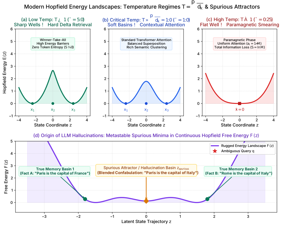
6.1 Temperature-Driven Regimes of Attention

The behavior of the attention layer is governed by the effective temperature $T = \sqrt{d_k}$:

1. High-Temperature Regime ($T \gg 1$, $\beta \to 0$):
   • The Log-Sum-Exp potential flattens into a single harmonic well:

$$\begin{aligned} \lim_{\beta \to 0} \operatorname{softmax}(\beta X^T \mathbf{z})_\mu = \frac{1}{M} \implies \mathbf{z}_{\mathrm{out}} = \frac{1}{M} \sum_{\mu=1}^M \mathbf{v}_\mu \end{aligned}$$

• Physical State: Paramagnetic Phase. Maximum entropy $S = \ln M$. The model outputs a global uniform average of all tokens, losing all positional and token-specific discrimination.

2. Low-Temperature Regime ($T \ll 1$, $\beta \to \infty$):
   • The softmax approaches the hard indicator (Dirac delta):

$$\begin{aligned} \lim_{\beta \to \infty} \operatorname{softmax}(\beta X^T \mathbf{z})_\mu = \begin{cases} 1 & \text{if } \mu = \operatorname{argmax}_\nu (\mathbf{x}_\nu^T \mathbf{z}) \\ 0 & \text{otherwise} \end{cases} \end{aligned}$$

• Physical State: Ferromagnetic Ground State. Zero entropy $S = 0$. Pure nearest-neighbor hard retrieval ($1$-NN search).

3. Intermediate Critical Regime ($T \sim \mathcal{O}(1)$):
   • Energy landscape exhibits multiple distinct, well-isolated local minima corresponding to individual keys, with moderate saddle points between semantically similar tokens.
   • Enables compositional reasoning: the output is a weighted superposition of relevant context tokens.

---

6.2 Spurious States and the Origin of LLM Hallucinations

What causes hallucinations in Large Language Models? In statistical physics, when memory patterns $\mathbf{x}_1, \mathbf{x}_2$ have non-zero mutual overlap $\mathbf{x}_1^T \mathbf{x}_2 \approx c > 0$, the energy landscape $E(\mathbf{z})$ develops metastable spurious minima at intermediate locations:

$$\begin{aligned} \mathbf{z}_{\mathrm{spurious}} \approx \frac{\mathbf{x}_1 + \mathbf{x}_2}{\|\mathbf{x}_1 + \mathbf{x}_2\|} \end{aligned}$$

When an autoregressive Transformer generates text, its query state $\mathbf{q}_t$ traverses the high-dimensional energy landscape. If the query falls into the basin of attraction of a spurious mixed state rather than a pure memory attractor, the attention output blends incompatible facts from disparate parts of the context window.

[!NOTE] Statistical Physics of Hallucination: Hallucination is not merely an optimization defect; it is the thermodynamic consequence of quenched crosstalk disorder creating metastable spurious attractors in the continuous Hopfield landscape when the token context density exceeds the local spin-glass threshold.

---

7. Spin-Glass Theory of In-Context Learning (ICL)

One of the most remarkable emergent phenomena in modern AI is In-Context Learning (ICL): without adjusting any model weights $\theta$, a pretrained Transformer can solve novel tasks at inference time given only a few demonstration examples in the prompt:

$$\begin{aligned} \mathcal{P} = \left( (x_1, y_1), (x_2, y_2), \dots, (x_L, y_L), x_{\mathrm{query}} \right) \end{aligned}$$

In a groundbreaking study, Li, Bai, and Huang (Physical Review E 2025) formulated In-Context Learning as a thermodynamic phase transition in a disordered spin glass.

7.1 Statistical Mechanics Formulation of ICL

Consider a sequence of $L$ demonstration pairs drawn from task distribution $\mathcal{T}_\alpha$. During pretraining, the Transformer is exposed to $P_{\mathrm{tasks}}$ distinct tasks drawn from an environment with task diversity $\gamma = P_{\mathrm{tasks}} / D_{\mathrm{param}}$.

Let the prompt tokens be represented by spin configurations $\mathbf{s}_1, \dots, \mathbf{s}_L$, interacting through the attention tensor $J_{ijkl} \sim W_Q \otimes W_K$. The effective Hamiltonian of the prompt processing is:

$$\begin{aligned} \mathcal{H}_{\mathrm{ICL}}(\mathbf{s}; \mathcal{T}_\alpha) = -\sum_{i, j=1}^L J_{ij}(\mathcal{T}_\alpha) \mathbf{s}_i \cdot \mathbf{s}_j - \sum_{i=1}^L \mathbf{h}_i \cdot \mathbf{s}_i \end{aligned}$$

The quenched disorder arises from two independent sources:

1. Intra-Task Sample Noise: Random variations in the demonstration pairs $(x_l, y_l)$.
2. Inter-Task Multi-Task Disorder: The variation across task definitions $\mathcal{T}_\alpha$.

---

7.2 The Task Condensation Phase Transition

Li et al. (2025) defined the Task Alignment Order Parameter:

$$\begin{aligned} q_{\mathrm{task}} = \frac{1}{L} \sum_{l=1}^L \mathbb{E}_{\mathcal{T}_\alpha} \left[ \langle \mathbf{s}_l \rangle_{\mathcal{H}} \cdot \mathbf{t}_\alpha \right] \end{aligned}$$

where $\mathbf{t}_\alpha$ is the true underlying task vector.

By applying the replica method to average over the multi-task disorder $\mathbb{E}_{\mathcal{T}}[\ln Z]$, they proved that the system undergoes a second-order thermodynamic phase transition as a function of pretraining task diversity $\gamma$:

$$\begin{aligned} q_{\mathrm{task}}(\gamma) = \begin{cases} 0 & \text{for } \gamma < \gamma_c \quad (\textbf{In-Weights Memorization Phase}) \\ C \cdot (\gamma - \gamma_c)^{1/2} & \text{for } \gamma \ge \gamma_c \quad (\textbf{In-Context Learning Phase}) \end{cases} \end{aligned}$$

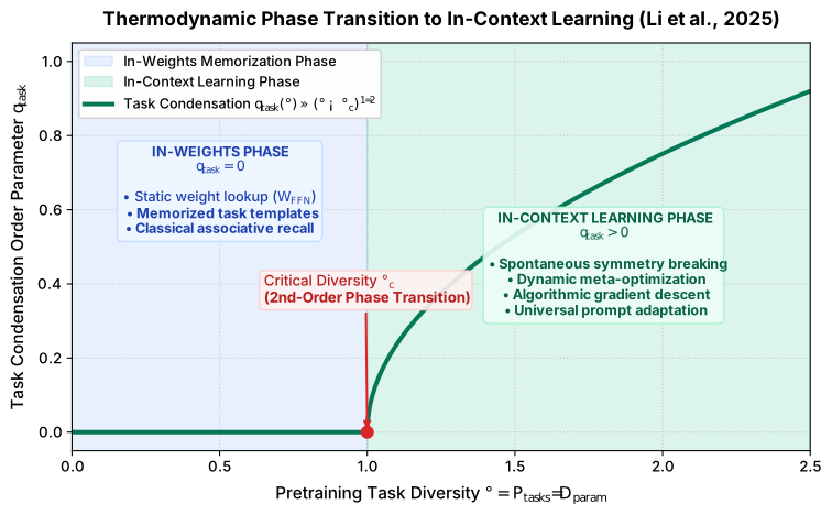Figure 4.3: The In-Context Learning Phase Transition. Below critical diversity $\gamma_c$, the attention mechanism acts as a simple associative memory retrieving pre-stored static task weights. Above $\gamma_c$, the system condenses into a dynamic meta-optimization state.

Physical Interpretation of the Phases:

1. In-Weights Phase ($\gamma < \gamma_c$): When pretraining data contains few tasks, the network memorizes individual task solutions directly into its static feed-forward weights ($W_{\mathrm{FFN}}$). The attention mechanism merely acts as a classical Hopfield network retrieving the nearest stored task template.
2. In-Context Learning Phase ($\gamma > \gamma_c$): High task diversity creates severe frustration in the static weights: no single set of static weights can satisfy all tasks simultaneously. To minimize total free energy, the system undergoes a symmetry-breaking condensation: the attention layers spontaneously configure themselves into an algorithmic in-context gradient descent optimizer (von Oswald et al., 2023; Dai et al., 2023).

---

7.3 Induction Heads as Non-Local Exchange Couplings

In mechanistic interpretability, induction heads (Olsson et al., 2022) are specific two-layer attention circuits that implement the prefix matching pattern: $[A][B] \dots [A] \longrightarrow [B]$

In our spin-glass framework, an induction head corresponds to an effective four-spin non-local exchange interaction:

$$\begin{aligned} H_{\mathrm{induction}} = -J_{\mathrm{ind}} \sum_{i < j} (\mathbf{s}_i \cdot \mathbf{s}_j) (\mathbf{s}_{i+1} \cdot \mathbf{s}_{j+1}) \end{aligned}$$

This Hamiltonian energetically rewards transitions where the continuation from state $j$ reproduces the continuation previously observed following state $i$, establishing long-range ferromagnetic order across distant sequence positions.

---

8. Frontier: Boltzmann Attention & Learnable Ising Couplings (2026)

While standard Transformer self-attention is equivalent to a continuous Modern Hopfield network, it suffers from a fundamental physical limitation: it is a mean-field model. The softmax operation treats each token's attention weight independently, subject only to a single global partition function normalization $\sum_\mu e^{\beta \mathbf{q} \mathbf{k}_\mu^T}$.

In 2026, researchers introduced Boltzmann Attention, which enriches the attention mechanism with explicit, learnable pairwise Ising interactions between tokens.

8.1 Mathematical Formulation of Boltzmann Attention

Let $\mathbf{a} = (a_1, a_2, \dots, a_N)^T \in \{0, 1\}^N$ be a binary attention selection vector indicating which context tokens are attended to ($a_i = 1$) or ignored ($a_i = 0$).

8.2 Mean-Field Equations for Cooperative Attention

Because exact evaluation of $\mathcal{Z}$ is NP-hard for arbitrary $J_{ij}$, the continuous relaxation $\bar{a}_i = \langle a_i \rangle \in [0, 1]$ is computed using Ising Mean-Field Self-Consistency Equations:

$$\begin{aligned} \bar{a}_i = \sigma\left( \frac{\mathbf{q}^T \mathbf{k}_i}{\sqrt{d_k}} - \theta_i + \sum_{j \ne i} J_{ij} \bar{a}_j \right) \end{aligned}$$

where $\sigma(u) = \frac{1}{1 + e^{-u}}$ is the sigmoid activation function.

$a_i^{(t+1)} = \sigma\left( \frac{q \cdot k_i}{\sqrt{d}} + \sum_{j \neq i} J_{ij} a_j^{(t)} - \theta_i \right)$

8.3 Physical Advantages of Boltzmann Attention:

1. Cooperative Chunking: Ferromagnetic couplings ($J_{ij} > 0$ for $|i-j| \le k$) encourage contiguous phrases or code blocks to be attended to as unified semantic chunks, eliminating fragmented attention.
2. First-Order Percolation Transition to Exact Sparsity: As the query strength varies, the attention weights undergo a sharp percolation phase transition from $\bar{a}_i = 0$ to $\bar{a}_i \approx 1$, achieving hardware-friendly exact $O(N)$ sparse attention without heuristics.
3. Suppression of Spurious Glassy Attractors: Antiferromagnetic long-range inhibition ($J_{ij} < 0$ for distant irrelevant tokens) actively suppresses the cross-talk noise responsible for LLM hallucinations.

---

9. Comprehensive Comparison: The Hopfield-Attention Family

To synthesize the theoretical developments covered in this chapter, the following table summarizes the structural and thermodynamic properties across all variants:

---

10. Summary and Core Takeaways

In this lecture, we established a rigorous mathematical bridge between statistical physics and deep learning architectures:

1. Spin Glasses and Frustration: The Sherrington-Kirkpatrick model reveals how quenched disorder and frustration generate complex, rugged free energy landscapes with exponentially many metastable states, described by Parisi's Replica Symmetry Breaking.
2. Classical Hopfield Networks: The AGS theory demonstrates that classical binary Hopfield networks are fundamentally limited to a linear capacity $M_{\max} \approx 0.138 N$, beyond which the network collapses into a disordered spin-glass phase.
3. Modern Continuous Hopfield Networks: By replacing quadratic energy functions with the convex Log-Sum-Exp potential, Modern Hopfield Networks achieve exponential storage capacity $M_{\max} \sim e^{c d}$ and converge in a single step via CCCP gradient descent.
4. Exact Equivalence to Self-Attention: Transformer self-attention is algebraically and dynamically identical to one update step of a continuous Modern Hopfield network, where queries are probing states, keys are stored attractors, softmax computes the Gibbs measure, and $\beta = 1/\sqrt{d_k}$ is the inverse temperature.
5. Phase Transitions in In-Context Learning: Pretraining on multi-task distributions acts as quenched disorder. Above a critical task diversity $\gamma_c$, the Transformer undergoes a second-order thermodynamic phase transition from in-weights memorization to dynamic in-context meta-optimization.
6. Boltzmann Attention: Incorporating learnable Ising couplings $J_{ij}$ moves attention beyond mean-field theory, enabling cooperative token chunking, exact first-order sparsity transitions, and suppression of spurious glassy hallucinations.

---

References & Further Reading

• Hopfield, J. J. (1982). Neural networks and physical systems with emergent collective computational abilities. Proceedings of the National Academy of Sciences (PNAS), 79(8), 2554–2558.
• Amit, D. J., Gutfreund, H., & Sompolinsky, H. (1985). Spin-glass models of neural networks. Physical Review A, 32(2), 1007.
• Sherrington, D., & Kirkpatrick, S. (1975). Solvable model of a spin-glass. Physical Review Letters, 35(26), 1792.
• Mézard, M., Parisi, G., & Virasoro, M. A. (1987). Spin Glass Theory and Beyond. World Scientific.
• Krotov, D., & Hopfield, J. J. (2016). Dense associative memory for pattern recognition. Advances in Neural Information Processing Systems (NeurIPS 2016).
• Demircigil, M., Heubeck, J., Ramsauer, H., & Toth, P. (2017). On a model of associative memory with huge storage capacity. Journal of Statistical Physics.
• Ramsauer, H., Schäfl, B., Lehner, J., et al. (2021). Hopfield Networks is All You Need. International Conference on Learning Representations (ICLR 2021).
• Vaswani, A., et al. (2017). Attention Is All You Need. NeurIPS 2017.
• Li, Z., Bai, Y., & Huang, H. (2025). Statistical physics of in-context learning in transformers. Physical Review E, 111(2), 024301.
• von Oswald, J., et al. (2023). Transformers learn in-context by gradient descent. ICML 2023.
• Olsson, C., et al. (2022). In-context learning and induction heads. Anthropic Transformer Circuits Thread.