CSE-41XX
Course Curriculum

1. Foundations: Gibbs Distributions, Softmax & Energy-Based Models

Microstates vs macrostates, Jaynes' Maximum Entropy derivation of the Boltzmann/Gibbs measure, exact equivalence with temperature-scaled softmax, and training Energy-Based Models in modern generative AI.

1. Introduction: The Bridge Between Statistical Physics and Generative AI

At first glance, classical statistical mechanics and modern generative machine learning appear to address disparate disciplines. The former was developed in the late 19th century by Ludwig Boltzmann, James Clerk Maxwell, and Josiah Willard Gibbs to explain how macroscopic thermodynamic observables—such as temperature, pressure, and heat capacity—emerge deterministically from the stochastic interactions of N1023N \sim 10^{23} microscopic atoms. The latter was developed by computer scientists to model complex, high-dimensional probability distributions over natural language tokens, image pixels, protein structures, and neural network weights.

Yet beneath their domain-specific terminologies, both fields solve the exact same mathematical problem:

The Fundamental Problem of Large Systems

Given an exponentially or uncountably large configuration space S\mathcal{S} and a scalar cost/energy function E:SRE: \mathcal{S} \to \mathbb{R}, what is the least-biased, mathematically principled probability distribution p(σ)p(\sigma) over states σS\sigma \in \mathcal{S} that satisfies macroscopic empirical constraints?

In physics, this question leads directly to the Boltzmann-Gibbs distribution p(σ)eβE(σ)p(\sigma) \propto e^{-\beta E(\sigma)}. In deep learning, this identical formula appears everywhere:

  • The Softmax activation function with temperature T=1/βT = 1/\beta in autoregressive Transformer language models (GPT-4, Llama 3, Claude 3.7).
  • Energy-Based Models (EBMs) and score-based generative models where probability densities are parameterized via unnormalized deep neural networks pθ(x)=1ZθeEθ(x)p_\theta(x) = \frac{1}{Z_\theta} e^{-E_\theta(x)}.
  • The optimal policy in Reinforcement Learning from Human Feedback (RLHF) and Direct Preference Optimization (DPO), where policy distributions form exact Gibbs measures parameterized by reward functions.
  • Modern Discrete Diffusion Models (such as SEDD and LLaDA) operating via discrete score matching over vocabulary spaces.

This chapter establishes the rigorous foundations of statistical physics required for modern deep learning. We build from microstates and macrostates to Jaynes' Maximum Entropy Principle, derive the canonical Gibbs measure from first principles, prove its equivalence to temperature-scaled softmax, analyze the training dynamics of Energy-Based Models, and explore sequence-level residual EBMs and energy-compositional controllable generation.


2. Microstates, Macrostates, and Phase Space

A central concept in statistical mechanics is the distinction between the complete microscopic description of a system and its low-dimensional macroscopic observation.

2.1 Discrete State Spaces

Consider a physical system composed of NN discrete components or a machine learning model operating on discrete sequences.

Classical Physics: The Ising Spin System

In a lattice of NN magnetic dipoles (spins), a microstate σ\sigma specifies the exact orientation of every individual spin:

σ=(s1,s2,,sN){1,+1}N\sigma = (s_1, s_2, \dots, s_N) \in \{-1, +1\}^N

The microstate space S={1,+1}N\mathcal{S} = \{-1, +1\}^N contains S=2N|\mathcal{S}| = 2^N discrete configurations. For a macroscopic sample of matter where N1023N \sim 10^{23}, the number of microstates is 210232^{10^{23}}, a quantity vastly exceeding the number of elementary particles in the observable universe (108010^{80}).

Natural Language Processing: Token Sequences

In an autoregressive Large Language Model with vocabulary V\mathcal{V} (where typically V32,000|\mathcal{V}| \approx 32{,}000 to 128,000128{,}000), a sequence y\mathbf{y} of length LL represents a discrete microstate:

y=(y1,y2,,yL)VL\mathbf{y} = (y_1, y_2, \dots, y_L) \in \mathcal{V}^L

For a context window of L=2048L = 2048 tokens and V=32,000|\mathcal{V}| = 32{,}000, the discrete configuration space has cardinality:

S=VL=(32,000)2048109,229|\mathcal{S}| = |\mathcal{V}|^L = (32{,}000)^{2048} \approx 10^{9{,}229}

No computer can enumerate, normalize, or directly evaluate all possible microstates in S\mathcal{S}.

Macrostates and Multiplicity

A macrostate is defined by a small set of macroscopic observables M(σ)M(\sigma) that summarize the system without tracking microscopic coordinates:

  • In physics: The total energy E(σ)=i,jJijsisjihisiE(\sigma) = -\sum_{\langle i,j \rangle} J_{ij} s_i s_j - \sum_i h_i s_i, or the net magnetization M(σ)=i=1NsiM(\sigma) = \sum_{i=1}^N s_i.
  • In NLP: The semantic topic, sentiment label y{+1,1}y \in \{+1, -1\}, syntactic grammaticality, or total sequence cross-entropy loss.

The multiplicity (or discrete density of states) Ω(E)\Omega(E) is the number of distinct microstates σS\sigma \in \mathcal{S} that produce the identical macroscopic energy EE:

Ω(E)=σSδ(E(σ)E)\Omega(E) = \sum_{\sigma \in \mathcal{S}} \delta(E(\sigma) - E)

where δ()\delta(\cdot) is the Kronecker delta. Ludwig Boltzmann discovered that the thermodynamic entropy SS of an isolated macrostate is proportional to the logarithm of its multiplicity:

S(E)=kBlnΩ(E)S(E) = k_B \ln \Omega(E)

where kB1.380649×1023 J/Kk_B \approx 1.380649 \times 10^{-23} \text{ J/K} is Boltzmann's constant (often set to kB=1k_B = 1 in information theory and machine learning).


2.2 Continuous State Spaces and Phase Space

When physical systems or neural representations are continuous, the microstate is represented by coordinates in a continuous manifold.

Classical Phase Space Γ\Gamma

For a system of NN classical point particles moving in dd-dimensional Euclidean space, a microstate is a single point x=(q,p)\mathbf{x} = (\mathbf{q}, \mathbf{p}) in a 2dN2dN-dimensional phase space Γ=R2dN\Gamma = \mathbb{R}^{2dN}:

q=(q1,q2,,qN)RdN,p=(p1,p2,,pN)RdN\mathbf{q} = (\mathbf{q}_1, \mathbf{q}_2, \dots, \mathbf{q}_N) \in \mathbb{R}^{dN}, \quad \mathbf{p} = (\mathbf{p}_1, \mathbf{p}_2, \dots, \mathbf{p}_N) \in \mathbb{R}^{dN}

where qi\mathbf{q}_i represents the position and pi=mvi\mathbf{p}_i = m \mathbf{v}_i represents the linear momentum of particle ii.

The differential volume element of phase space, nondimensionalized via Planck's constant hh and corrected for quantum indistinguishability of identical particles (the Gibbs factor 1/N!1/N!), is:

dΓ=ddNqddNphdNN!d\Gamma = \frac{d^{dN} \mathbf{q} \, d^{dN} \mathbf{p}}{h^{dN} N!}

The continuous density of states g(E)g(E) for a Hamiltonian H(q,p)H(\mathbf{q}, \mathbf{p}) is defined via the Dirac delta function:

g(E)=Γδ(H(q,p)E)dΓg(E) = \int_{\Gamma} \delta(H(\mathbf{q}, \mathbf{p}) - E) \, d\Gamma

Deep Learning: Continuous Latent Spaces and Diffusion Models

In continuous generative modeling (e.g., Score-based Diffusion Models, Continuous Normalizing Flows, and Variational Autoencoders), a microstate xRD\mathbf{x} \in \mathbb{R}^D represents an image, an audio waveform, or a continuous latent embedding zRd\mathbf{z} \in \mathbb{R}^d:

  • In Image Diffusion (DDPM / Score-SDE): D=C×H×WD = C \times H \times W (e.g., 3×512×5127.86×1053 \times 512 \times 512 \approx 7.86 \times 10^5 dimensions).
  • In Generative Flow Matching: The continuous trajectory xtRD\mathbf{x}_t \in \mathbb{R}^D is governed by a time-dependent vector field vθ(xt,t)v_\theta(\mathbf{x}_t, t).
  • The macrostate corresponds to class labels (e.g., "Image of a golden retriever"), style descriptors, or clip embeddings.

2.3 The Rosetta Stone: Statistical Mechanics \longleftrightarrow Deep Learning

To navigate the cross-disciplinary literature, we construct the exact translation table connecting physical statistical mechanics to machine learning and computer science concepts:

Concept / QuantityStatistical MechanicsMachine Learning & Deep Learning
MicrostateMicroscopic coordinate σS\sigma \in \mathcal{S} or (q,p)Γ(\mathbf{q}, \mathbf{p}) \in \GammaToken sequence yVL\mathbf{y} \in \mathcal{V}^L, image vector xRD\mathbf{x} \in \mathbb{R}^D, or model weights w\mathbf{w}
Energy FunctionHamiltonian H(σ)H(\sigma) or potential energy E(x)E(\mathbf{x})Negative logit zi-z_i, loss function L(θ)\mathcal{L}(\theta), or energy network Eθ(x)E_\theta(\mathbf{x})
MacrostateMacroscopic observables (E,V,N,M)(E, V, N, M)Class labels, prompt conditioning cc, semantic intent, dataset statistics
Density of StatesMultiplicity Ω(E)=σδ(E(σ)E)\Omega(E) = \sum_\sigma \delta(E(\sigma) - E)Volume of configuration space satisfying loss L(w)ϵ\mathcal{L}(\mathbf{w}) \le \epsilon
Inverse Temperatureβ=1kBT\beta = \frac{1}{k_B T}Inverse sampling temperature β=1/T\beta = 1/T in Softmax / LLM decoding
Gibbs / Boltzmann Measurep(σ)=1ZeβH(σ)p(\sigma) = \frac{1}{Z} e^{-\beta H(\sigma)}Temperature-scaled Softmax pi=ezi/Tjezj/Tp_i = \frac{e^{z_i / T}}{\sum_j e^{z_j / T}}
Partition FunctionZ(β)=σeβE(σ)=eβHdΓZ(\beta) = \sum_\sigma e^{-\beta E(\sigma)} = \int e^{-\beta H} d\GammaNormalization constant Zθ=eEθ(x)dxZ_\theta = \int e^{-E_\theta(\mathbf{x})} d\mathbf{x}, Softmax denominator
Free EnergyHelmholtz Free Energy F=1βlnZ=ETSF = -\frac{1}{\beta} \ln Z = \langle E \rangle - TSLog-Sum-Exp LSE(z)\operatorname{LSE}(\mathbf{z}), Negative Log Marginal Likelihood, Variational Free Energy
EntropyThermodynamic / Gibbs entropy S=kBpilnpiS = -k_B \sum p_i \ln p_iShannon Entropy H(p)=pilnpiH(p) = -\sum p_i \ln p_i, exploration bonus in RL / MaxEnt RL
Fluctuations & Heat CapacityCv=ET=β2Var(E)C_v = \frac{\partial \langle E \rangle}{\partial T} = \beta^2 \operatorname{Var}(E)Variance of gradients Var(L)\operatorname{Var}(\nabla \mathcal{L}), Hessian trace, Fisher Information Matrix

3. The Postulate of Equal A Priori Probabilities & Jaynes' MaxEnt Principle

How do we assign probabilities to microstates when our only empirical knowledge consists of macroscopic expectations?

3.1 The Microcanonical Ensemble & Equal A Priori Probabilities

For a completely isolated physical system with fixed total energy in the interval [E,E+δE][E, E + \delta E], total volume VV, and particle number NN, we possess zero information distinguishing one compatible microstate from another.

Postulate of Equal A Priori Probabilities

An isolated system in thermodynamic equilibrium is equally likely to be found in any of its accessible microstates. That is, for all microstates σS\sigma \in \mathcal{S} compatible with macrostate (E,V,N)(E, V, N):

p(σ)={1Ω(E)if E(σ)[E,E+δE]0otherwisep(\sigma) = \begin{cases} \frac{1}{\Omega(E)} & \text{if } E(\sigma) \in [E, E + \delta E] \\ 0 & \text{otherwise} \end{cases}

In classical mechanics, this postulate is justified dynamically via Liouville's Theorem (which proves that phase space volume is preserved under Hamiltonian time evolution) and the Ergodic Hypothesis (which asserts that over long timescales, the time average of an observable along a single trajectory equals its phase-space ensemble average):

limT1T0TA(q(t),p(t))dt=ΓA(q,p)pmicro(q,p)dΓ\lim_{\mathcal{T} \to \infty} \frac{1}{\mathcal{T}} \int_0^{\mathcal{T}} A(\mathbf{q}(t), \mathbf{p}(t)) \, dt = \int_{\Gamma} A(\mathbf{q}, \mathbf{p}) \, p_{\text{micro}}(\mathbf{q}, \mathbf{p}) \, d\Gamma

3.2 Jaynes' Principle of Maximum Entropy (MaxEnt)

In two seminal 1957 papers, Edwin T. Jaynes revolutionized statistical mechanics by reinterpreting it not as a purely physical theory of mechanical trajectories, but as a general framework for optimal statistical inference under incomplete information.

Suppose we have a discrete random variable XX taking values in X={x1,x2,,xK}\mathcal{X} = \{x_1, x_2, \dots, x_K\}. We do not know the true distribution p=(p1,p2,,pK)p = (p_1, p_2, \dots, p_K), but we have measured MM macroscopic expectation values:

Ep[fm(X)]=k=1Kpkfm(xk)=αm,m{1,2,,M}\mathbb{E}_p [f_m(X)] = \sum_{k=1}^K p_k f_m(x_k) = \alpha_m, \quad \forall m \in \{1, 2, \dots, M\}

where M<KM < K, meaning the system of equations is severely underdetermined with infinitely many valid probability distributions.

The Principle of Maximum Entropy (Jaynes, 1957)

The uniquely unbiased probability distribution pp that incorporates the known constraints while remaining maximally agnostic about all other unmeasured degrees of freedom is the distribution that maximizes the Shannon entropy:

H(p)=k=1KpklnpkH(p) = - \sum_{k=1}^K p_k \ln p_k

Any other choice of distribution implicitly assumes extra, unjustified information.


4. First-Principles Derivation of the Boltzmann/Gibbs Distribution

We now present the rigorous step-by-step mathematical derivation of the Boltzmann/Gibbs distribution using the method of Lagrange multipliers under the Jaynes MaxEnt framework.

4.1 The Constrained Optimization Problem

Let S={1,2,,K}\mathcal{S} = \{1, 2, \dots, K\} be the index set of all microstates. Each microstate iSi \in \mathcal{S} has an associated microscopic energy EiRE_i \in \mathbb{R}.

We seek the probability vector p=(p1,p2,,pK)T\mathbf{p} = (p_1, p_2, \dots, p_K)^T that solves:

maxpH(p)=i=1Kpilnpisubject toC1:i=1Kpi=1(Total probability axiom)C2:i=1KpiEi=U(Prescribed internal energy expectation E=U)C3:pi0,i{1,,K}(Non-negativity)\begin{aligned} \max_{\mathbf{p}} \quad & H(\mathbf{p}) = -\sum_{i=1}^K p_i \ln p_i \\ \text{subject to} \quad & C_1: \sum_{i=1}^K p_i = 1 \quad \text{(Total probability axiom)} \\ & C_2: \sum_{i=1}^K p_i E_i = U \quad \text{(Prescribed internal energy expectation $\langle E \rangle = U$)} \\ & C_3: p_i \ge 0, \quad \forall i \in \{1, \dots, K\} \quad \text{(Non-negativity)} \end{aligned}

4.2 Step-by-Step Lagrange Multiplier Derivation

Step 1: Construct the Lagrangian Function

We introduce Lagrange multipliers λ0R\lambda_0 \in \mathbb{R} for the normalization constraint C1C_1, and βR\beta \in \mathbb{R} for the energy constraint C2C_2. The Lagrangian L(p,λ0,β)\mathcal{L}(\mathbf{p}, \lambda_0, \beta) is:

L(p1,,pK,λ0,β)=i=1Kpilnpiλ0(i=1Kpi1)β(i=1KpiEiU)\mathcal{L}(p_1, \dots, p_K, \lambda_0, \beta) = -\sum_{i=1}^K p_i \ln p_i - \lambda_0 \left( \sum_{i=1}^K p_i - 1 \right) - \beta \left( \sum_{i=1}^K p_i E_i - U \right)

Step 2: Compute Stationary Points

We take the partial derivative of L\mathcal{L} with respect to an arbitrary microstate probability pkp_k:

Lpk=pk[pklnpk]λ0pkpkβEkpkpk\frac{\partial \mathcal{L}}{\partial p_k} = \frac{\partial}{\partial p_k} \left[ -p_k \ln p_k \right] - \lambda_0 \frac{\partial p_k}{\partial p_k} - \beta E_k \frac{\partial p_k}{\partial p_k}

Evaluating the derivatives using the product rule:

pk[pklnpk]=lnpkpk1pk=lnpk1\frac{\partial}{\partial p_k} \left[ -p_k \ln p_k \right] = -\ln p_k - p_k \cdot \frac{1}{p_k} = -\ln p_k - 1

Setting the gradient to zero for stationarity:

Lpk=lnpk1λ0βEk=0\frac{\partial \mathcal{L}}{\partial p_k} = - \ln p_k - 1 - \lambda_0 - \beta E_k = 0

Step 3: Solve for the Microstate Probability pkp_k

Rearranging the algebraic equation:

lnpk=(1+λ0)βEk\ln p_k = -(1 + \lambda_0) - \beta E_k

Exponentiating both sides:

pk=exp((1+λ0))exp(βEk)p_k = \exp\left( -(1 + \lambda_0) \right) \cdot \exp\left( -\beta E_k \right)

Notice that because exp()>0\exp(\cdot) > 0, the non-negativity constraint pk>0p_k > 0 is automatically satisfied for all finite β\beta and EkE_k.

Step 4: Eliminate the Multiplier λ0\lambda_0 via Normalization

We enforce the total probability constraint k=1Kpk=1\sum_{k=1}^K p_k = 1:

k=1Kpk=k=1Kexp((1+λ0))exp(βEk)=1\sum_{k=1}^K p_k = \sum_{k=1}^K \exp\left( -(1 + \lambda_0) \right) \exp\left( -\beta E_k \right) = 1

Factoring out the constant scalar term exp((1+λ0))\exp(-(1 + \lambda_0)):

exp((1+λ0))[k=1Kexp(βEk)]=1\exp\left( -(1 + \lambda_0) \right) \left[ \sum_{k=1}^K \exp\left( -\beta E_k \right) \right] = 1

We define the sum over all unnormalized Boltzmann weights as the Canonical Partition Function Z(β)Z(\beta):

Z(β)k=1Kexp(βEk)Z(\beta) \equiv \sum_{k=1}^K \exp(-\beta E_k)

Therefore:

exp((1+λ0))=1Z(β)\exp(-(1 + \lambda_0)) = \frac{1}{Z(\beta)}

Substituting this back into our expression for pkp_k yields the Boltzmann/Gibbs distribution:

The Canonical Boltzmann / Gibbs Measure

pi=1Z(β)eβEi=eβEij=1KeβEjp_i = \frac{1}{Z(\beta)} e^{-\beta E_i} = \frac{e^{-\beta E_i}}{\sum_{j=1}^K e^{-\beta E_j}}

where β=1kBT\beta = \frac{1}{k_B T} is the thermodynamic inverse temperature and Z(β)Z(\beta) is the partition function (Zustandssumme).


4.3 Physical and Mathematical Properties of the Partition Function

The partition function Z(β)Z(\beta) is not merely an arbitrary normalization constant; it is the cumulant generating function of the energy distribution and encapsulates all thermodynamic properties of the system.

1. Free Energy Connection

In thermodynamics, the Helmholtz Free Energy FF represents the maximum usable work obtainable from a closed system at constant temperature:

FUTS=E1βH(p)F \equiv U - TS = \langle E \rangle - \frac{1}{\beta} H(p)

Using the Gibbs distribution, we compute the entropy:

H(p)=ipiln(eβEiZ)=ipi(βEilnZ)=βipiEi+lnZipi=βE+lnZ\begin{aligned} H(p) &= -\sum_i p_i \ln\left(\frac{e^{-\beta E_i}}{Z}\right) = -\sum_i p_i (-\beta E_i - \ln Z) \\ &= \beta \sum_i p_i E_i + \ln Z \sum_i p_i = \beta \langle E \rangle + \ln Z \end{aligned}

Rearranging gives the fundamental identity connecting statistical mechanics to thermodynamics:

1βlnZ=E1βH(p)=F-\frac{1}{\beta} \ln Z = \langle E \rangle - \frac{1}{\beta} H(p) = F

Hence:

F(β)=1βlnZ(β)    Z(β)=eβF(β)F(\beta) = -\frac{1}{\beta} \ln Z(\beta) \iff Z(\beta) = e^{-\beta F(\beta)}

2. Expected Energy as the First Log-Derivative

The expected internal energy U=EU = \langle E \rangle is obtained by differentiating lnZ\ln Z:

lnZβ=1ZZβ=1Zβ[ieβEi]=1Zi(Ei)eβEi=iEipi=E\frac{\partial \ln Z}{\partial \beta} = \frac{1}{Z} \frac{\partial Z}{\partial \beta} = \frac{1}{Z} \frac{\partial}{\partial \beta}\left[\sum_i e^{-\beta E_i}\right] = \frac{1}{Z} \sum_i (-E_i) e^{-\beta E_i} = - \sum_i E_i p_i = -\langle E \rangle

Thus:

E=lnZ(β)β\langle E \rangle = -\frac{\partial \ln Z(\beta)}{\partial \beta}

3. Energy Fluctuations and Heat Capacity

Differentiating a second time yields the energy variance:

2lnZβ2=β[1ZiEieβEi]=1Z2(Zβ)iEieβEi1Zi(Ei2)eβEi=E(E)+iEi2pi=E2E2=Varp(E)\begin{aligned} \frac{\partial^2 \ln Z}{\partial \beta^2} &= \frac{\partial}{\partial \beta} \left[ -\frac{1}{Z} \sum_i E_i e^{-\beta E_i} \right] \\ &= \frac{1}{Z^2} \left(\frac{\partial Z}{\partial \beta}\right) \sum_i E_i e^{-\beta E_i} - \frac{1}{Z} \sum_i (-E_i^2) e^{-\beta E_i} \\ &= -\langle E \rangle (-\langle E \rangle) + \sum_i E_i^2 p_i \\ &= \langle E^2 \rangle - \langle E \rangle^2 = \operatorname{Var}_p(E) \end{aligned}

In physics, this variance is directly proportional to the heat capacity at constant volume Cv=UTC_v = \frac{\partial U}{\partial T}:

Var(E)=2lnZβ2=Eβ=kBT2Cv\operatorname{Var}(E) = \frac{\partial^2 \ln Z}{\partial \beta^2} = -\frac{\partial \langle E \rangle}{\partial \beta} = k_B T^2 C_v

Key Insight: Fluctuations Reveal Response

Equation Var(E)=kBT2Cv\operatorname{Var}(E) = k_B T^2 C_v is an elementary instance of the Fluctuation-Dissipation Theorem: the equilibrium microscopic fluctuations of an observable (Var(E)\operatorname{Var}(E)) dictate the macroscopic linear response of the system to external perturbations (Cv=dU/dTC_v = dU/dT).


5. Exact Mathematical Equivalence: Gibbs Distributions & Softmax with Temperature

We now establish the direct, 1-to-1 isomorphism between the Boltzmann/Gibbs measure of statistical physics and the Softmax activation function used across modern neural architectures.

Statistical Mechanics ConceptDeep Learning / LLM CounterpartMathematical Isomorphism
Microstate Energy (EiE_i)Negative Logit (zi-z_i)EiziE_i \longleftrightarrow -z_i
Inverse Temperature (β=1kBT\beta = \frac{1}{k_B T})Inverse Softmax Temperature (β=1T\beta = \frac{1}{T})β1T\beta \longleftrightarrow \frac{1}{T}
Partition Function (Z(β)Z(\beta))Softmax Normalizing DenominatorZ=ieβEiiezi/TZ = \sum_i e^{-\beta E_i} \longleftrightarrow \sum_i e^{z_i / T}
Helmholtz Free Energy (F=1βlnZF = -\frac{1}{\beta} \ln Z)Negative Log-Sum-Exp (LSE(z)-\text{LSE}(z))FTlniezi/TF \longleftrightarrow -T \ln \sum_i e^{z_i / T}
Gibbs-Boltzmann DistributionSoftmax Output Distributionpi=eβEiZpi=ezi/Tjezj/Tp_i = \frac{e^{-\beta E_i}}{Z} \longleftrightarrow p_i = \frac{e^{z_i / T}}{\sum_j e^{z_j / T}}

5.1 The Equivalence Map

Let z=(z1,z2,,zK)TRK\mathbf{z} = (z_1, z_2, \dots, z_K)^T \in \mathbb{R}^K be a vector of unnormalized network outputs (logits) over KK discrete classes (or tokens). Let T>0T > 0 denote the scalar temperature parameter.

Define the microscopic energy of state ii as the negative logit:

EiziE_i \equiv -z_i

Define the thermodynamic inverse temperature as:

β1T(setting kB=1)\beta \equiv \frac{1}{T} \quad (\text{setting } k_B = 1)

Substituting these definitions directly into the Boltzmann distribution:

pi=eβEij=1KeβEj=e(1/T)(zi)j=1Ke(1/T)(zj)=exp(zi/T)j=1Kexp(zj/T)softmax(zT)ip_i = \frac{e^{-\beta E_i}}{\sum_{j=1}^K e^{-\beta E_j}} = \frac{e^{-(1/T)(-z_i)}}{\sum_{j=1}^K e^{-(1/T)(-z_j)}} = \frac{\exp(z_i / T)}{\sum_{j=1}^K \exp(z_j / T)} \equiv \operatorname{softmax}\left(\frac{\mathbf{z}}{T}\right)_i

The mathematical objects are identical:

  1. Softmax is the Gibbs distribution where logits are negative energies.
  2. The neural network acts as an energy parameterization engine: higher logit zi    z_i \iff lower energy Ei    E_i \iff higher probability pip_i.
  3. The Log-Sum-Exp operator is the negative free energy (times temperature):
LSE(z)=ln(j=1Kezj)=lnZ=βF\operatorname{LSE}(\mathbf{z}) = \ln \left( \sum_{j=1}^K e^{z_j} \right) = \ln Z = -\beta F

5.2 Asymptotic Temperature Regimes in Generative LLMs

In Large Language Models, when generating the next token ytsoftmax(zt/T)y_t \sim \operatorname{softmax}(\mathbf{z}_t / T), tuning TT controls the physical thermodynamic state of the generation process:

1. Zero Temperature Limit (T0+    βT \to 0^+ \iff \beta \to \infty): Ground State Condensation

In physics, as T0T \to 0, all thermal fluctuations freeze out, and the system condenses with probability 1 into its ground state (the configuration with minimal energy Emin=minkEkE_{\min} = \min_k E_k):

limT0+pi=limβeβEijeβEj=limβeβ(EiEmin)jeβ(EjEmin)\lim_{T \to 0^+} p_i = \lim_{\beta \to \infty} \frac{e^{-\beta E_i}}{\sum_j e^{-\beta E_j}} = \lim_{\beta \to \infty} \frac{e^{-\beta (E_i - E_{\min})}}{\sum_j e^{-\beta (E_j - E_{\min})}}

Let G={kEk=Emin}\mathcal{G} = \{k \mid E_k = E_{\min}\} be the set of degenerate ground states. For any state iGi \notin \mathcal{G}, EiEmin>0E_i - E_{\min} > 0, so eβ(EiEmin)0e^{-\beta(E_i - E_{\min})} \to 0 as β\beta \to \infty. Thus:

limT0+pi={1Gif iG    zi=maxjzj0otherwise\lim_{T \to 0^+} p_i = \begin{cases} \frac{1}{|\mathcal{G}|} & \text{if } i \in \mathcal{G} \iff z_i = \max_j z_j \\ 0 & \text{otherwise} \end{cases}

In LLM generation, this corresponds to Greedy Decoding (argmaxizi\operatorname{argmax}_i z_i). The entropy collapses to S0S \to 0, eliminating output diversity.

2. Infinite Temperature Limit (T    β0+T \to \infty \iff \beta \to 0^+): Pure Maximum Entropy

In physics, as TT \to \infty, thermal fluctuations completely overwhelm the energetic potential barrier. Expanding the exponential to first order:

eβEi=1βEi+O(β2)β01e^{-\beta E_i} = 1 - \beta E_i + \mathcal{O}(\beta^2) \xrightarrow{\beta \to 0} 1

Therefore:

limTpi=1j=1K1=1K\lim_{T \to \infty} p_i = \frac{1}{\sum_{j=1}^K 1} = \frac{1}{K}

In LLMs, TT \to \infty produces uniform random sampling across the entire vocabulary V\mathcal{V}, yielding complete semantic incoherence and maximum entropy H=lnVH = \ln |\mathcal{V}|.

3. Intermediate Sampling Techniques: Truncated Canonical Support

To prevent sampling from the high-energy (low-probability) tail of the Gibbs distribution while preserving local diversity, practitioners use:

  • Top-kk Sampling: Truncates the state space to the kk lowest-energy microstates: Sk={irank(Ei)k}\mathcal{S}_k = \{i \mid \operatorname{rank}(E_i) \le k\}.
  • Top-pp (Nucleus) Sampling (Holtzman et al., 2020): Restricts sampling to the minimal set of microstates SpS\mathcal{S}_p \subset \mathcal{S} whose cumulative Gibbs mass satisfies:
iSppip\sum_{i \in \mathcal{S}_p} p_i \ge p

6. Energy-Based Models (EBMs) in Machine Learning

Having established that parameterized distributions over configurations x\mathbf{x} naturally take the form of a Gibbs measure, we now examine Energy-Based Models (EBMs) in machine learning.

6.1 Formulation of Unnormalized Generative Density

An Energy-Based Model parameterizes a continuous or discrete probability distribution over data xRD\mathbf{x} \in \mathbb{R}^D via an unnormalized scalar energy function Eθ(x):RDRE_\theta(\mathbf{x}): \mathbb{R}^D \to \mathbb{R} parameterized by neural network weights θ\theta:

Definition: Energy-Based Model

pθ(x)=exp(Eθ(x))Z(θ)p_\theta(\mathbf{x}) = \frac{\exp(-E_\theta(\mathbf{x}))}{Z(\theta)}

where the partition function Z(θ)Z(\theta) is the integral over the entire continuous data manifold:

Z(θ)=Xexp(Eθ(x))dxZ(\theta) = \int_{\mathcal{X}} \exp(-E_\theta(\mathbf{x})) \, d\mathbf{x}

Why EBMs? Architectural Freedom and Compositionality

Unlike other generative frameworks, EBMs impose zero architectural restrictions:

  1. Autoregressive Models require causal masking and chain-rule factorization p(x)=tp(xtx<t)p(\mathbf{x}) = \prod_{t} p(x_t \mid x_{<t}), imposing fixed generation orderings.
  2. Normalizing Flows require invertible transformations with tractable Jacobian determinants det(fx)\det(\frac{\partial f}{\partial \mathbf{x}}), restricting expressivity.
  3. VAEs require tractable approximate posteriors qϕ(zx)q_\phi(\mathbf{z} \mid \mathbf{x}) and suffer from blurry reconstructions due to loose variational bounds.
  4. GANs require unstable adversarial min-max optimization (minGmaxDV(D,G)\min_G \max_D V(D,G)).
  5. EBMs allow Eθ(x)E_\theta(\mathbf{x}) to be any arbitrary deep neural network mapping inputs to a scalar energy value. Crucially, EBMs allow exact compositionality: combining independent constraints amounts to simply summing their energies:
p(x)e(E1(x)+E2(x))=eE1(x)eE2(x)p(\mathbf{x}) \propto e^{-(E_1(\mathbf{x}) + E_2(\mathbf{x}))} = e^{-E_1(\mathbf{x})} e^{-E_2(\mathbf{x})}

6.2 The Fundamental Challenge: The Intractable Partition Function

The primary challenge of EBMs is that the partition function Z(θ)=RDeEθ(x)dxZ(\theta) = \int_{\mathbb{R}^D} e^{-E_\theta(\mathbf{x})} d\mathbf{x} is a high-dimensional integral. In dimensions D100D \ge 100, computing Z(θ)Z(\theta) numerically via grid quadrature requires O(KD)\mathcal{O}(K^D) evaluations, which is fundamentally computationally intractable (#P-hard).


6.3 Maximum Likelihood Learning and the Positive / Negative Phase

Suppose we are given an empirical dataset D={x1,x2,,xN}\mathcal{D} = \{\mathbf{x}_1, \mathbf{x}_2, \dots, \mathbf{x}_N\} sampled i.i.d. from true data distribution pdata(x)p_{\text{data}}(\mathbf{x}). We wish to train the parameters θ\theta of Eθ(x)E_\theta(\mathbf{x}) by maximizing the average log-likelihood:

L(θ)=Expdata[lnpθ(x)]=Expdata[Eθ(x)lnZ(θ)]\mathcal{L}(\theta) = \mathbb{E}_{\mathbf{x} \sim p_{\text{data}}} [\ln p_\theta(\mathbf{x})] = \mathbb{E}_{\mathbf{x} \sim p_{\text{data}}} \left[ -E_\theta(\mathbf{x}) - \ln Z(\theta) \right]

We now compute the exact gradient θL(θ)\nabla_\theta \mathcal{L}(\theta).

Derivation of the Log-Likelihood Gradient

The gradient decomposes into two terms:

θL(θ)=Expdata[θEθ(x)]θlnZ(θ)\nabla_\theta \mathcal{L}(\theta) = -\mathbb{E}_{\mathbf{x} \sim p_{\text{data}}} [\nabla_\theta E_\theta(\mathbf{x})] - \nabla_\theta \ln Z(\theta)

We evaluate the gradient of the log partition function:

θlnZ(θ)=1Z(θ)θZ(θ)=1Z(θ)θ[XeEθ(x)dx]=1Z(θ)Xθ[eEθ(x)]dx=1Z(θ)X(θEθ(x))eEθ(x)dx=X[eEθ(x)Z(θ)]θEθ(x)dx=Xpθ(x)θEθ(x)dx=Expθ[θEθ(x)]\begin{aligned} \nabla_\theta \ln Z(\theta) &= \frac{1}{Z(\theta)} \nabla_\theta Z(\theta) \\ &= \frac{1}{Z(\theta)} \nabla_\theta \left[ \int_{\mathcal{X}} e^{-E_\theta(\mathbf{x}')} \, d\mathbf{x}' \right] \\ &= \frac{1}{Z(\theta)} \int_{\mathcal{X}} \nabla_\theta \left[ e^{-E_\theta(\mathbf{x}')} \right] \, d\mathbf{x}' \\ &= \frac{1}{Z(\theta)} \int_{\mathcal{X}} \left( -\nabla_\theta E_\theta(\mathbf{x}') \right) e^{-E_\theta(\mathbf{x}')} \, d\mathbf{x}' \\ &= -\int_{\mathcal{X}} \left[ \frac{e^{-E_\theta(\mathbf{x}')}}{Z(\theta)} \right] \nabla_\theta E_\theta(\mathbf{x}') \, d\mathbf{x}' \\ &= -\int_{\mathcal{X}} p_\theta(\mathbf{x}') \nabla_\theta E_\theta(\mathbf{x}') \, d\mathbf{x}' \\ &= -\mathbb{E}_{\mathbf{x}' \sim p_\theta} [\nabla_\theta E_\theta(\mathbf{x}')] \end{aligned}

Substituting this back yields the central theorem of Energy-Based Learning:

The Fundamental EBM Gradient Equation

θL(θ)=Expdata[θEθ(x)]Positive Phase (Data)+Expθ[θEθ(x)]Negative Phase (Model Samples)\nabla_\theta \mathcal{L}(\theta) = \underbrace{-\mathbb{E}_{\mathbf{x} \sim p_{\text{data}}} [\nabla_\theta E_\theta(\mathbf{x})]}_{\text{Positive Phase (Data)}} + \underbrace{\mathbb{E}_{\mathbf{x}' \sim p_\theta} [\nabla_\theta E_\theta(\mathbf{x}')]}_{\text{Negative Phase (Model Samples)}}

Physical and Intuitive Interpretation:

  1. The Positive Phase: Takes true observed data points xpdata\mathbf{x} \sim p_{\text{data}} and updates θ\theta to push their energy down (Eθ(x)    pθ(x)E_\theta(\mathbf{x}) \downarrow \implies p_\theta(\mathbf{x}) \uparrow).
  2. The Negative Phase: Generates ungrounded "fantasies" or "hallucinations" xpθ\mathbf{x}' \sim p_\theta from the current model distribution and updates θ\theta to pull their energy up (Eθ(x)    pθ(x)E_\theta(\mathbf{x}') \uparrow \implies p_\theta(\mathbf{x}') \downarrow).
  3. Stationary Equilibrium: Learning converges when the expectations match:
Expdata[θEθ(x)]=Expθ[θEθ(x)]    pθ(x)=pdata(x)\mathbb{E}_{\mathbf{x} \sim p_{\text{data}}} [\nabla_\theta E_\theta(\mathbf{x})] = \mathbb{E}_{\mathbf{x}' \sim p_\theta} [\nabla_\theta E_\theta(\mathbf{x}')] \iff p_\theta(\mathbf{x}) = p_{\text{data}}(\mathbf{x})

6.4 Sampling Algorithms: SGLD & Contrastive Divergence

To compute the negative phase gradient Expθ[θEθ(x)]\mathbb{E}_{\mathbf{x}' \sim p_\theta}[\nabla_\theta E_\theta(\mathbf{x}')], we must sample configurations xpθ(x)eEθ(x)\mathbf{x}' \sim p_\theta(\mathbf{x}) \propto e^{-E_\theta(\mathbf{x})}.

Stochastic Gradient Langevin Dynamics (SGLD)

In continuous spaces xRD\mathbf{x} \in \mathbb{R}^D, we sample from the Gibbs measure using Langevin dynamics (Welling & Teh, 2011; Du & Mordatch, 2019):

xk+1=xkϵ2xEθ(xk)+ϵξk,ξkN(0,ID)\mathbf{x}_{k+1} = \mathbf{x}_k - \frac{\epsilon}{2} \nabla_\mathbf{x} E_\theta(\mathbf{x}_k) + \sqrt{\epsilon} \mathbf{\xi}_k, \quad \mathbf{\xi}_k \sim \mathcal{N}(0, I_D)

where:

  • ϵ2xEθ(xk)-\frac{\epsilon}{2} \nabla_\mathbf{x} E_\theta(\mathbf{x}_k) is the deterministic drift pulling the sample toward low-energy basins.
  • ϵξk\sqrt{\epsilon} \mathbf{\xi}_k is the Brownian thermal noise injecting entropy to explore the entire phase space.

As step size ϵ0\epsilon \to 0 and steps KK \to \infty, the stationary distribution of the Markov chain converges exactly to the Gibbs distribution pθ(x)eEθ(x)p_\theta(\mathbf{x}) \propto e^{-E_\theta(\mathbf{x})}.

Contrastive Divergence (CD-kk) and Replay Buffers

Running full SGLD to equilibrium at every gradient step is prohibitively slow. Contrastive Divergence (CDkCD_k, Hinton 2002) initializes the Langevin Markov chain at data points x0pdata\mathbf{x}_0 \sim p_{\text{data}} and runs only kk steps (k550k \approx 5 - 50). Modern deep EBMs (Du & Mordatch, 2019) maintain a persistent Replay Buffer of past negative samples to allow chains to mix across training iterations.


6.5 Circumventing the Partition Function: Score Matching

Can we train an Energy-Based Model without evaluating or approximating Z(θ)Z(\theta) at all?

Aapo Hyvärinen (2005) introduced Score Matching, which optimizes the vector field of log-density derivatives (the score function):

sθ(x)xlnpθ(x)\mathbf{s}_\theta(\mathbf{x}) \equiv \nabla_\mathbf{x} \ln p_\theta(\mathbf{x})

Applying the definition of an EBM:

sθ(x)=x[Eθ(x)lnZ(θ)]=xEθ(x)xlnZ(θ)=0 (indep. of x)=xEθ(x)\mathbf{s}_\theta(\mathbf{x}) = \nabla_\mathbf{x} \left[ -E_\theta(\mathbf{x}) - \ln Z(\theta) \right] = -\nabla_\mathbf{x} E_\theta(\mathbf{x}) - \underbrace{\nabla_\mathbf{x} \ln Z(\theta)}_{= 0 \text{ (indep. of } \mathbf{x})} = -\nabla_\mathbf{x} E_\theta(\mathbf{x})

Fundamental Property of Score Matching

The score function sθ(x)=xEθ(x)\mathbf{s}_\theta(\mathbf{x}) = -\nabla_\mathbf{x} E_\theta(\mathbf{x}) is strictly independent of the partition function Z(θ)Z(\theta)! Differentiating with respect to the data coordinate x\mathbf{x} eliminates the normalization constant entirely.

Explicit Score Matching (ESM) Objective

Score matching minimizes the expected squared Fisher divergence between the model score and true data score:

JESM(θ)=12Expdata[xlnpθ(x)xlnpdata(x)22]J_{\text{ESM}}(\theta) = \frac{1}{2} \mathbb{E}_{\mathbf{x} \sim p_{\text{data}}} \left[ \left\| \nabla_\mathbf{x} \ln p_\theta(\mathbf{x}) - \nabla_\mathbf{x} \ln p_{\text{data}}(\mathbf{x}) \right\|_2^2 \right]

Using integration by parts (assuming pdata(x)xlnpθ(x)0p_{\text{data}}(\mathbf{x}) \nabla_\mathbf{x} \ln p_\theta(\mathbf{x}) \to 0 at the domain boundary), Hyvärinen proved this is equivalent to:

JSM(θ)=Expdata[12xEθ(x)22Tr(x2Eθ(x))]J_{\text{SM}}(\theta) = \mathbb{E}_{\mathbf{x} \sim p_{\text{data}}} \left[ \frac{1}{2} \left\| \nabla_\mathbf{x} E_\theta(\mathbf{x}) \right\|_2^2 - \operatorname{Tr}\left( \nabla_\mathbf{x}^2 E_\theta(\mathbf{x}) \right) \right]

where Tr(x2Eθ(x))=d=1D2Eθ(x)xd2\operatorname{Tr}(\nabla_\mathbf{x}^2 E_\theta(\mathbf{x})) = \sum_{d=1}^D \frac{\partial^2 E_\theta(\mathbf{x})}{\partial x_d^2} is the trace of the Hessian (the Laplacian ΔEθ(x)\Delta E_\theta(\mathbf{x})).

This remarkable identity gave birth to modern Score-based Generative Models and Diffusion SDEs (Song & Ermon, 2019; Song et al., 2021; Ho et al., 2020), which we will explore in detail in Chapter 6.


6.6 Noise Contrastive Estimation (NCE)

Another approach to bypass Z(θ)Z(\theta) is Noise Contrastive Estimation (NCE) (Gutmann & Hyvärinen, 2010). NCE treats the unnormalized model as a binary classifier trained to distinguish true data xpdata\mathbf{x} \sim p_{\text{data}} from synthetic noise generated by a known noise distribution yq(x)\mathbf{y} \sim q(\mathbf{x}):

p(D=1x)=pθ(x)pθ(x)+νq(x)=eEθ(x)ceEθ(x)c+νq(x)p(D=1 \mid \mathbf{x}) = \frac{p_\theta(\mathbf{x})}{p_\theta(\mathbf{x}) + \nu q(\mathbf{x})} = \frac{e^{-E_\theta(\mathbf{x}) - c}}{e^{-E_\theta(\mathbf{x}) - c} + \nu q(\mathbf{x})}

where the log partition function c=lnZ(θ)c = \ln Z(\theta) is simply treated as a single scalar learnable parameter alongside θ\theta. As the number of noise samples ν\nu \to \infty, the parameter estimates θ^\hat{\theta} and c^\hat{c} converge to their true maximum likelihood values.


7. Case Studies in NLP: Residual EBMs & Controllable Energy Generation

How do these statistical mechanics principles manifest in state-of-the-art Natural Language Processing?

7.1 Sequence-Level Residual EBMs for Text (Deng et al., ICLR 2020)

Standard autoregressive language models pAR(y)=t=1Lp(yty<t)p_{\text{AR}}(\mathbf{y}) = \prod_{t=1}^L p(y_t \mid y_{<t}) decompose text generation into a sequence of local, myopic token predictions. While highly efficient for sampling, autoregressive models struggle with global, sequence-level constraints (e.g., long-range discourse coherence, holistic semantic consistency).

Deng et al. (ICLR 2020) proposed Residual Energy-Based Models for text. Instead of training an EBM from scratch, they define the joint sequence distribution as a product of a pre-trained autoregressive base model pAR(yx)p_{\text{AR}}(\mathbf{y} \mid \mathbf{x}) and a non-autoregressive residual energy function Eθ(x,y)E_\theta(\mathbf{x}, \mathbf{y}):

Residual EBM Parameterization

pθ(yx)=pAR(yx)exp(Eθ(x,y))Zθ(x)p_\theta(\mathbf{y} \mid \mathbf{x}) = \frac{p_{\text{AR}}(\mathbf{y} \mid \mathbf{x}) \exp(-E_\theta(\mathbf{x}, \mathbf{y}))}{Z_\theta(\mathbf{x})}

where the conditional partition function is:

Zθ(x)=yVLpAR(yx)exp(Eθ(x,y))Z_\theta(\mathbf{x}) = \sum_{\mathbf{y}' \in \mathcal{V}^L} p_{\text{AR}}(\mathbf{y}' \mid \mathbf{x}) \exp(-E_\theta(\mathbf{x}, \mathbf{y}'))

Why Residual Parameterization Succeeds

  1. Division of Labor: pAR(yx)p_{\text{AR}}(\mathbf{y} \mid \mathbf{x}) captures local grammar, syntax, and short-range transitions. Eθ(x,y)E_\theta(\mathbf{x}, \mathbf{y}) (parameterized via bidirectional Transformers like BERT or RoBERTa) inspects the entire sequence simultaneously to evaluate holistic coherence.
  2. Tractable Importance Sampling: Because pARp_{\text{AR}} is already close to the data distribution, we can draw candidate sequences y(1),,y(K)pAR(yx)\mathbf{y}^{(1)}, \dots, \mathbf{y}^{(K)} \sim p_{\text{AR}}(\mathbf{y} \mid \mathbf{x}) and compute self-normalized importance sampling estimates of the conditional partition function:
Zθ(x)=EypAR[exp(Eθ(x,y))]1Kk=1Kexp(Eθ(x,y(k)))Z_\theta(\mathbf{x}) = \mathbb{E}_{\mathbf{y}' \sim p_{\text{AR}}} \left[ \exp(-E_\theta(\mathbf{x}, \mathbf{y}')) \right] \approx \frac{1}{K} \sum_{k=1}^K \exp(-E_\theta(\mathbf{x}, \mathbf{y}^{(k)}))

Training is conducted stably via Noise Contrastive Estimation (NCE), yielding state-of-the-art results on text summarization and machine translation.


7.2 Controllable Generation via Energy Composition: "Mix and Match" (ACL 2022)

In controllable text generation, we wish to sample text y\mathbf{y} that satisfies multiple simultaneous attribute constraints:

  1. High fluency / grammaticality (base language model ELME_{\text{LM}}).
  2. Positive sentiment (EsentimentE_{\text{sentiment}}).
  3. Specific topic / domain, e.g. "Quantum Computing" (EtopicE_{\text{topic}}).
  4. Strict safety / anti-toxicity constraint (EsafetyE_{\text{safety}}).

Fine-tuning a separate 70B parameter model for every possible permutation of attributes is computationally prohibitive. Statistical mechanics provides an elegant, zero-shot solution through the composition of energy functions (Product of Experts, Hinton 2002; Mireshghallah et al., ACL 2022):

Energy Composition Formula

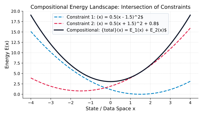
p(y)exp(Etotal(y))p(\mathbf{y}) \propto \exp\left( - E_{\text{total}}(\mathbf{y}) \right)

where the total energy is a linear combination of independent modular energy discriminators:

Etotal(y)=ELM(y)+λ1Esentiment(y)+λ2Etopic(y)+λ3Esafety(y)E_{\text{total}}(\mathbf{y}) = E_{\text{LM}}(\mathbf{y}) + \lambda_1 E_{\text{sentiment}}(\mathbf{y}) + \lambda_2 E_{\text{topic}}(\mathbf{y}) + \lambda_3 E_{\text{safety}}(\mathbf{y})

Compositional Energy Landscape: Intersection of Constraints

Discrete Gibbs Sampling / MCMC in Token Space

Because text is discrete, continuous SGLD cannot be applied directly. Instead, "Mix and Match" applies Discrete Gibbs / Metropolis-Hastings Sampling:

  1. Initialize with an arbitrary sequence y(0)=(y1,,yL)\mathbf{y}^{(0)} = (y_1, \dots, y_L).
  2. At step tt, select a random token position j{1,,L}j \in \{1, \dots, L\}.
  3. Mask token yjy_j and propose a replacement token vVv \in \mathcal{V} using a masked language model (e.g. BERT) proposal distribution q(vyj)q(v \mid \mathbf{y}_{-j}).
  4. Accept the candidate sequence y=(y1,,v,,yL)\mathbf{y}' = (y_1, \dots, v, \dots, y_L) with Metropolis-Hastings acceptance probability:
α(yy)=min(1,exp(Etotal(y))exp(Etotal(y))q(yjyj)q(vyj))\alpha(\mathbf{y} \to \mathbf{y}') = \min\left(1, \, \frac{\exp(-E_{\text{total}}(\mathbf{y}'))}{\exp(-E_{\text{total}}(\mathbf{y}))} \cdot \frac{q(\mathbf{y}_j \mid \mathbf{y}'_{-j})}{q(v \mid \mathbf{y}_{-j})} \right)

This allows non-autoregressive, plug-and-play controllable steering of pre-trained models without modifying a single model weight.


7.3 Direct Preference Optimization (DPO): An Exact Gibbs Partition Cancellation

A preview of Lecture 2: In Reinforcement Learning from Human Feedback (RLHF), the goal is to find an optimal policy πθ(yx)\pi_\theta(y \mid x) maximizing expected human reward r(x,y)r(x,y) regularized by KL-divergence to a reference model πref(yx)\pi_{\text{ref}}(y \mid x):

maxπExD,yπ(x)[r(x,y)]βDKL(π(yx)πref(yx))\max_{\pi} \mathbb{E}_{x \sim \mathcal{D}, y \sim \pi(\cdot \mid x)} [r(x,y)] - \beta D_{\text{KL}}(\pi(y \mid x) \,\|\, \pi_{\text{ref}}(y \mid x))

Solving this constrained optimization problem analytically (as we will prove in Chapter 2) yields an exact Gibbs distribution:

π(yx)=1Z(x)πref(yx)exp(1βr(x,y))\pi^*(y \mid x) = \frac{1}{Z(x)} \pi_{\text{ref}}(y \mid x) \exp\left( \frac{1}{\beta} r(x,y) \right)

where Z(x)=yπref(yx)exp(1βr(x,y))Z(x) = \sum_{y} \pi_{\text{ref}}(y \mid x) \exp(\frac{1}{\beta} r(x,y)) is the intractable partition function.

In Direct Preference Optimization (DPO) (Rafailov et al., NeurIPS 2023), taking the logarithm of this exact Gibbs relationship allows expressing the latent reward function directly in terms of policy probabilities:

r(x,y)=βlnπ(yx)πref(yx)+βlnZ(x)r(x,y) = \beta \ln \frac{\pi^*(y \mid x)}{\pi_{\text{ref}}(y \mid x)} + \beta \ln Z(x)

When evaluating the pairwise Bradley-Terry preference probability p(ywylx)=σ(r(x,yw)r(x,yl))p(y_w \succ y_l \mid x) = \sigma(r(x, y_w) - r(x, y_l)), the partition functions cancel each other out identically:

r(x,yw)r(x,yl)=βlnπθ(ywx)πref(ywx)βlnπθ(ylx)πref(ylx)r(x, y_w) - r(x, y_l) = \beta \ln \frac{\pi_\theta(y_w \mid x)}{\pi_{\text{ref}}(y_w \mid x)} - \beta \ln \frac{\pi_\theta(y_l \mid x)}{\pi_{\text{ref}}(y_l \mid x)}

This allows optimizing human preferences without training a reward model and without sampling from the negative phase of the Gibbs distribution during training.


8. Summary & Key Mathematical Identities

To synthesize the theoretical foundations established in Lecture 1, we summarize the core mathematical formulas and their computational roles:

Mathematical ConceptFormal ExpressionOperational Meaning in AI / Physics
MaxEnt Shannon EntropyH(p)=ipilnpiH(p) = -\sum_{i} p_i \ln p_iMeasure of uncertainty; maximization yields least-biased distributions
Boltzmann / Gibbs Measurepi=1ZeβEip_i = \frac{1}{Z} e^{-\beta E_i}Equilibrium probability of state ii under energy constraint
Canonical Partition FunctionZ(β)=ieβEiZ(\beta) = \sum_i e^{-\beta E_i}Normalization factor; cumulant generating function of energy
Helmholtz Free EnergyF=1βlnZ=ETSF = -\frac{1}{\beta} \ln Z = \langle E \rangle - TSMinimum achievable energy discounted by entropic capacity
Expected Internal EnergyE=lnZβ\langle E \rangle = -\frac{\partial \ln Z}{\partial \beta}First moment of energy under the canonical ensemble
Energy FluctuationsVar(E)=2lnZβ2=kBT2Cv\operatorname{Var}(E) = \frac{\partial^2 \ln Z}{\partial \beta^2} = k_B T^2 C_vSecond central moment; connects fluctuations to heat capacity
Temperature Softmaxpi=exp(zi/T)jexp(zj/T)p_i = \frac{\exp(z_i/T)}{\sum_j \exp(z_j/T)}Exact Gibbs measure with Ei=ziE_i = -z_i and β=1/T\beta = 1/T
Log-Sum-Exp OperatorLSE(z)=lnjezj=βF\operatorname{LSE}(\mathbf{z}) = \ln \sum_j e^{z_j} = -\beta FFree energy in deep networks; smooth approximation to max\max
EBM Likelihood GradientθL=Epdata[θEθ]+Epθ[θEθ]\nabla_\theta \mathcal{L} = -\mathbb{E}_{p_{\text{data}}}[\nabla_\theta E_\theta] + \mathbb{E}_{p_\theta}[\nabla_\theta E_\theta]Push down energy of data (positive) and pull up energy of fantasies (negative)
Score Functions(x)=xlnp(x)=xE(x)\mathbf{s}(\mathbf{x}) = \nabla_\mathbf{x} \ln p(\mathbf{x}) = -\nabla_\mathbf{x} E(\mathbf{x})Vector field pointing toward high density; completely independent of ZZ

9. Analytical Exercise Problems

To master the mathematical tools derived in this chapter, work through the following complete analytical problems.

Problem 1: Maximum Entropy with Multiple Feature Constraints

Prompt: Let XX be a discrete random variable taking values in X\mathcal{X}. Suppose we measure MM independent macroscopic feature functions f(X)=(f1(X),f2(X),,fM(X))T\mathbf{f}(X) = (f_1(X), f_2(X), \dots, f_M(X))^T such that E[fm(X)]=αm\mathbb{E}[f_m(X)] = \alpha_m for m=1,,Mm=1, \dots, M. Prove that the Maximum Entropy distribution is a member of the general exponential family:

pθ(x)=1Z(θ)exp(m=1Mθmfm(x))p_{\boldsymbol{\theta}}(x) = \frac{1}{Z(\boldsymbol{\theta})} \exp\left( \sum_{m=1}^M \theta_m f_m(x) \right)

where θ=(θ1,,θM)T\boldsymbol{\theta} = (\theta_1, \dots, \theta_M)^T are the Lagrange multipliers.

Solution: We formulate the Lagrangian with multipliers λ0\lambda_0 for normalization and θ=(θ1,,θM)T\boldsymbol{\theta} = (\theta_1, \dots, \theta_M)^T for the MM expectation constraints:

L(p,λ0,θ)=xp(x)lnp(x)λ0(xp(x)1)+m=1Mθm(xp(x)fm(x)αm)\mathcal{L}(p, \lambda_0, \boldsymbol{\theta}) = -\sum_{x} p(x) \ln p(x) - \lambda_0 \left( \sum_x p(x) - 1 \right) + \sum_{m=1}^M \theta_m \left( \sum_x p(x) f_m(x) - \alpha_m \right)

Differentiating with respect to p(x)p(x) and setting to zero:

Lp(x)=lnp(x)1λ0+m=1Mθmfm(x)=0\frac{\partial \mathcal{L}}{\partial p(x)} = -\ln p(x) - 1 - \lambda_0 + \sum_{m=1}^M \theta_m f_m(x) = 0

Solving for p(x)p(x):

p(x)=exp((1+λ0))exp(m=1Mθmfm(x))p(x) = \exp(-(1 + \lambda_0)) \exp\left( \sum_{m=1}^M \theta_m f_m(x) \right)

Enforcing normalization xp(x)=1\sum_x p(x) = 1 gives e1+λ0=xexp(m=1Mθmfm(x))Z(θ)e^{1+\lambda_0} = \sum_x \exp\left( \sum_{m=1}^M \theta_m f_m(x) \right) \equiv Z(\boldsymbol{\theta}). Hence:

pθ(x)=1Z(θ)exp(θTf(x))p_{\boldsymbol{\theta}}(x) = \frac{1}{Z(\boldsymbol{\theta})} \exp\left( \boldsymbol{\theta}^T \mathbf{f}(x) \right) \quad \blacksquare

Problem 2: Score Matching Hessian Trace Identity

Prompt: Prove that for any smooth probability density pdata(x)p_{\text{data}}(\mathbf{x}) and model pθ(x)=1ZθeEθ(x)p_\theta(\mathbf{x}) = \frac{1}{Z_\theta} e^{-E_\theta(\mathbf{x})}, the expected squared score error:

J(θ)=12RDpdata(x)xlnpθ(x)xlnpdata(x)22dxJ(\theta) = \frac{1}{2} \int_{\mathbb{R}^D} p_{\text{data}}(\mathbf{x}) \left\| \nabla_\mathbf{x} \ln p_\theta(\mathbf{x}) - \nabla_\mathbf{x} \ln p_{\text{data}}(\mathbf{x}) \right\|_2^2 d\mathbf{x}

is equal (up to a constant independent of θ\theta) to:

JSM(θ)=RDpdata(x)[12xEθ(x)22Tr(x2Eθ(x))]dxJ_{\text{SM}}(\theta) = \int_{\mathbb{R}^D} p_{\text{data}}(\mathbf{x}) \left[ \frac{1}{2} \|\nabla_\mathbf{x} E_\theta(\mathbf{x})\|_2^2 - \operatorname{Tr}(\nabla_\mathbf{x}^2 E_\theta(\mathbf{x})) \right] d\mathbf{x}

Solution: Expanding the squared L2L_2 norm inside the integral:

J(θ)=12pdata(x)(xlnpθ(x)222xlnpθ(x),xlnpdata(x)+xlnpdata(x)22)dx\begin{aligned} J(\theta) &= \frac{1}{2} \int p_{\text{data}}(\mathbf{x}) \left( \|\nabla_\mathbf{x} \ln p_\theta(\mathbf{x})\|_2^2 - 2 \langle \nabla_\mathbf{x} \ln p_\theta(\mathbf{x}), \nabla_\mathbf{x} \ln p_{\text{data}}(\mathbf{x}) \rangle + \|\nabla_\mathbf{x} \ln p_{\text{data}}(\mathbf{x})\|_2^2 \right) d\mathbf{x} \end{aligned}

The third term xlnpdata(x)22\|\nabla_\mathbf{x} \ln p_{\text{data}}(\mathbf{x})\|_2^2 does not depend on θ\theta and can be dropped as a constant CC.

Now consider the cross term. Notice that pdata(x)xlnpdata(x)=xpdata(x)p_{\text{data}}(\mathbf{x}) \nabla_\mathbf{x} \ln p_{\text{data}}(\mathbf{x}) = \nabla_\mathbf{x} p_{\text{data}}(\mathbf{x}). Thus:

Icross=RDxlnpθ(x),xpdata(x)dx=d=1DRDlnpθ(x)xdpdata(x)xddxI_{\text{cross}} = -\int_{\mathbb{R}^D} \langle \nabla_\mathbf{x} \ln p_\theta(\mathbf{x}), \nabla_\mathbf{x} p_{\text{data}}(\mathbf{x}) \rangle d\mathbf{x} = -\sum_{d=1}^D \int_{\mathbb{R}^D} \frac{\partial \ln p_\theta(\mathbf{x})}{\partial x_d} \frac{\partial p_{\text{data}}(\mathbf{x})}{\partial x_d} d\mathbf{x}

Applying multidimensional integration by parts to each coordinate xdx_d:

lnpθ(x)xdpdata(x)xddxd=[pdata(x)lnpθ(x)xd]pdata(x)2lnpθ(x)xd2dxd\int_{-\infty}^\infty \frac{\partial \ln p_\theta(\mathbf{x})}{\partial x_d} \frac{\partial p_{\text{data}}(\mathbf{x})}{\partial x_d} dx_d = \left[ p_{\text{data}}(\mathbf{x}) \frac{\partial \ln p_\theta(\mathbf{x})}{\partial x_d} \right]_{-\infty}^\infty - \int_{-\infty}^\infty p_{\text{data}}(\mathbf{x}) \frac{\partial^2 \ln p_\theta(\mathbf{x})}{\partial x_d^2} dx_d

Assuming boundary conditions pdata(x)0p_{\text{data}}(\mathbf{x}) \to 0 as x\|\mathbf{x}\| \to \infty, the boundary term vanishes. Summing over all dimensions d{1,,D}d \in \{1, \dots, D\}:

Icross=RDpdata(x)d=1D2lnpθ(x)xd2dx=RDpdata(x)Tr(x2lnpθ(x))dxI_{\text{cross}} = \int_{\mathbb{R}^D} p_{\text{data}}(\mathbf{x}) \sum_{d=1}^D \frac{\partial^2 \ln p_\theta(\mathbf{x})}{\partial x_d^2} d\mathbf{x} = \int_{\mathbb{R}^D} p_{\text{data}}(\mathbf{x}) \operatorname{Tr}\left( \nabla_\mathbf{x}^2 \ln p_\theta(\mathbf{x}) \right) d\mathbf{x}

Substituting lnpθ(x)=Eθ(x)lnZθ\ln p_\theta(\mathbf{x}) = -E_\theta(\mathbf{x}) - \ln Z_\theta:

  • xlnpθ(x)=xEθ(x)    xlnpθ(x)22=xEθ(x)22\nabla_\mathbf{x} \ln p_\theta(\mathbf{x}) = -\nabla_\mathbf{x} E_\theta(\mathbf{x}) \implies \|\nabla_\mathbf{x} \ln p_\theta(\mathbf{x})\|_2^2 = \|\nabla_\mathbf{x} E_\theta(\mathbf{x})\|_2^2
  • x2lnpθ(x)=x2Eθ(x)    Tr(x2lnpθ(x))=Tr(x2Eθ(x))\nabla_\mathbf{x}^2 \ln p_\theta(\mathbf{x}) = -\nabla_\mathbf{x}^2 E_\theta(\mathbf{x}) \implies \operatorname{Tr}(\nabla_\mathbf{x}^2 \ln p_\theta(\mathbf{x})) = -\operatorname{Tr}(\nabla_\mathbf{x}^2 E_\theta(\mathbf{x}))

Combining terms gives:

JSM(θ)=Expdata[12xEθ(x)22Tr(x2Eθ(x))]J_{\text{SM}}(\theta) = \mathbb{E}_{\mathbf{x} \sim p_{\text{data}}} \left[ \frac{1}{2} \|\nabla_\mathbf{x} E_\theta(\mathbf{x})\|_2^2 - \operatorname{Tr}(\nabla_\mathbf{x}^2 E_\theta(\mathbf{x})) \right] \quad \blacksquare

Problem 3: Exact Bradley-Terry Partition Function Cancellation in DPO

Prompt: Consider two sequences ywy_w (preferred) and yly_l (dispreferred) conditioned on prompt xx. Under the Bradley-Terry preference model, the probability that ywyly_w \succ y_l is given by:

p(ywylx)=σ(r(x,yw)r(x,yl))=11+e(r(x,yw)r(x,yl))p(y_w \succ y_l \mid x) = \sigma(r^*(x, y_w) - r^*(x, y_l)) = \frac{1}{1 + e^{-(r^*(x, y_w) - r^*(x, y_l))}}

Assume the optimal Gibbs policy is π(yx)=1Z(x)πref(yx)exp(1βr(x,y))\pi^*(y \mid x) = \frac{1}{Z(x)} \pi_{\text{ref}}(y \mid x) \exp\left( \frac{1}{\beta} r^*(x, y) \right). Show that the Bradley-Terry preference likelihood can be expressed entirely in terms of the ratio of policies π\pi^* and πref\pi_{\text{ref}}, without any dependence on the partition function Z(x)Z(x).

Solution: From the optimal Gibbs policy formula:

π(yx)=πref(yx)exp(1βr(x,y))Z(x)\pi^*(y \mid x) = \frac{\pi_{\text{ref}}(y \mid x) \exp\left(\frac{1}{\beta} r^*(x,y)\right)}{Z(x)}

Taking the natural logarithm of both sides:

lnπ(yx)=lnπref(yx)+1βr(x,y)lnZ(x)\ln \pi^*(y \mid x) = \ln \pi_{\text{ref}}(y \mid x) + \frac{1}{\beta} r^*(x,y) - \ln Z(x)

Rearranging to isolate the ground-truth reward r(x,y)r^*(x,y):

r(x,y)=βln(π(yx)πref(yx))+βlnZ(x)r^*(x,y) = \beta \ln\left(\frac{\pi^*(y \mid x)}{\pi_{\text{ref}}(y \mid x)}\right) + \beta \ln Z(x)

Now compute the reward difference between the winning completion ywy_w and losing completion yly_l:

r(x,yw)r(x,yl)=[βln(π(ywx)πref(ywx))+βlnZ(x)][βln(π(ylx)πref(ylx))+βlnZ(x)]=βln(π(ywx)πref(ywx))βln(π(ylx)πref(ylx))+(βlnZ(x)βlnZ(x))=0=βln[π(ywx)πref(ywx)πref(ylx)π(ylx)]\begin{aligned} r^*(x, y_w) - r^*(x, y_l) &= \left[ \beta \ln\left(\frac{\pi^*(y_w \mid x)}{\pi_{\text{ref}}(y_w \mid x)}\right) + \beta \ln Z(x) \right] - \left[ \beta \ln\left(\frac{\pi^*(y_l \mid x)}{\pi_{\text{ref}}(y_l \mid x)}\right) + \beta \ln Z(x) \right] \\ &= \beta \ln\left(\frac{\pi^*(y_w \mid x)}{\pi_{\text{ref}}(y_w \mid x)}\right) - \beta \ln\left(\frac{\pi^*(y_l \mid x)}{\pi_{\text{ref}}(y_l \mid x)}\right) + \underbrace{\left( \beta \ln Z(x) - \beta \ln Z(x) \right)}_{= 0} \\ &= \beta \ln \left[ \frac{\pi^*(y_w \mid x)}{\pi_{\text{ref}}(y_w \mid x)} \cdot \frac{\pi_{\text{ref}}(y_l \mid x)}{\pi^*(y_l \mid x)} \right] \end{aligned}

Substituting this reward difference directly into the sigmoid function:

p(ywylx)=σ(βlnπ(ywx)πref(ywx)βlnπ(ylx)πref(ylx))p(y_w \succ y_l \mid x) = \sigma\left( \beta \ln \frac{\pi^*(y_w \mid x)}{\pi_{\text{ref}}(y_w \mid x)} - \beta \ln \frac{\pi^*(y_l \mid x)}{\pi_{\text{ref}}(y_l \mid x)} \right)

The partition function Z(x)Z(x) has cancelled identically, enabling direct preference optimization without reward modeling or MCMC sampling. \blacksquare


10. References & Further Reading

On this page

1. Introduction: The Bridge Between Statistical Physics and Generative AI2. Microstates, Macrostates, and Phase Space2.1 Discrete State SpacesClassical Physics: The Ising Spin SystemNatural Language Processing: Token SequencesMacrostates and Multiplicity2.2 Continuous State Spaces and Phase SpaceClassical Phase Space Γ\GammaDeep Learning: Continuous Latent Spaces and Diffusion Models2.3 The Rosetta Stone: Statistical Mechanics \longleftrightarrow Deep Learning3. The Postulate of Equal A Priori Probabilities & Jaynes' MaxEnt Principle3.1 The Microcanonical Ensemble & Equal A Priori Probabilities3.2 Jaynes' Principle of Maximum Entropy (MaxEnt)4. First-Principles Derivation of the Boltzmann/Gibbs Distribution4.1 The Constrained Optimization Problem4.2 Step-by-Step Lagrange Multiplier DerivationStep 1: Construct the Lagrangian FunctionStep 2: Compute Stationary PointsStep 3: Solve for the Microstate Probability pkp_kStep 4: Eliminate the Multiplier λ0\lambda_0 via Normalization4.3 Physical and Mathematical Properties of the Partition Function1. Free Energy Connection2. Expected Energy as the First Log-Derivative3. Energy Fluctuations and Heat Capacity5. Exact Mathematical Equivalence: Gibbs Distributions & Softmax with Temperature5.1 The Equivalence Map5.2 Asymptotic Temperature Regimes in Generative LLMs1. Zero Temperature Limit (T0+    βT \to 0^+ \iff \beta \to \infty): Ground State Condensation2. Infinite Temperature Limit (T    β0+T \to \infty \iff \beta \to 0^+): Pure Maximum Entropy3. Intermediate Sampling Techniques: Truncated Canonical Support6. Energy-Based Models (EBMs) in Machine Learning6.1 Formulation of Unnormalized Generative DensityWhy EBMs? Architectural Freedom and Compositionality6.2 The Fundamental Challenge: The Intractable Partition Function6.3 Maximum Likelihood Learning and the Positive / Negative PhaseDerivation of the Log-Likelihood GradientPhysical and Intuitive Interpretation:6.4 Sampling Algorithms: SGLD & Contrastive DivergenceStochastic Gradient Langevin Dynamics (SGLD)Contrastive Divergence (CD-kk) and Replay Buffers6.5 Circumventing the Partition Function: Score MatchingExplicit Score Matching (ESM) Objective6.6 Noise Contrastive Estimation (NCE)7. Case Studies in NLP: Residual EBMs & Controllable Energy Generation7.1 Sequence-Level Residual EBMs for Text (Deng et al., ICLR 2020)Why Residual Parameterization Succeeds7.2 Controllable Generation via Energy Composition: "Mix and Match" (ACL 2022)Discrete Gibbs Sampling / MCMC in Token Space7.3 Direct Preference Optimization (DPO): An Exact Gibbs Partition Cancellation8. Summary & Key Mathematical Identities9. Analytical Exercise ProblemsProblem 1: Maximum Entropy with Multiple Feature ConstraintsProblem 2: Score Matching Hessian Trace IdentityProblem 3: Exact Bradley-Terry Partition Function Cancellation in DPO10. References & Further Reading