6. Langevin Dynamics, Score-Based SDEs & Generative Diffusion

Generative modeling in modern machine learning represents a profound computational realization of non-equilibrium statistical mechanics. At its core, the problem of generative modeling asks: How can we transform an uninformative, high-entropy prior distribution (such as isotropic Gaussian noise or a sequence of mask tokens) into a highly structured, low-entropy data distribution (such as natural images, protein conformations, or coherent text)?

In classical physics, this problem is mirrored by the study of thermal relaxation, Brownian motion, and time-reversal symmetry in stochastic systems. In this chapter, we develop the complete mathematical continuum that connects the 1905 Einstein-Langevin theory of Brownian motion to continuous-time score-based Stochastic Differential Equations (Score-SDEs), Denoising Diffusion Probabilistic Models (DDPM), and modern Discrete Diffusion Large Language Models (SEDD, LLaDA).

---

The Physical Paradigm of Generative Modeling

Before diving into formal stochastic calculus, let us construct the conceptual dictionary bridging Classical Statistical Mechanics and Modern Deep Generative Diffusion.

---

Microscopic Foundations: Brownian Motion & The Classical Langevin Equation

Physical Setup: Pollen Grains and Thermal Solvent

Consider a macroscopic or mesoscopic particle of mass $m$ and position $x(t) \in \mathbb{R}^d$ suspended in a fluid solvent at absolute temperature $T$. The solvent consists of an astronomical number of fluid molecules ($N \sim 10^{23}$) undergoing rapid, chaotic thermal motion.

The microscopic collisions exerted by the fluid on the particle can be partitioned into two distinct physical effects across timescales:

1. Macroscopic Systematic Friction (Dissipation): A mean drag force opposing the velocity $\dot{x}(t) = v(t)$, modeled via Stokes' drag law as $-\gamma v(t)$, where $\gamma > 0$ is the friction coefficient.
2. Microscopic Random Kicks (Fluctuation): A rapidly fluctuating stochastic force $\eta(t)$ arising from individual, instantaneous molecular collisions.

Newton's second law yields the Classical Langevin Equation (Paul Langevin, 1908):

$$m \frac{d^2 x(t)}{dt^2} = -\gamma \frac{dx(t)}{dt} + \eta(t)$$

Equivalently, writing in terms of velocity $v(t) = \dot{x}(t)$:

$$m \frac{dv(t)}{dt} = -\gamma v(t) + \eta(t)$$

Statistical Properties of Thermal White Noise

Because molecular collisions occur on a picosecond timescale ($\tau_c \sim 10^{-13}\text{ s}$), vastly faster than the relaxation timescale of the mesoscopic particle ($\tau_r = m/\gamma \sim 10^{-7}\text{ s}$), we model $\eta(t)$ as a stationary, Gaussian white noise stochastic process:

1. Zero Mean: $$\mathbb{E}[\eta(t)] = 0$$
2. Delta-Correlated in Time (Markovian Memoryless Limit): $$\mathbb{E}\left[\eta(t) \eta(t')^T\right] = 2 D_v \delta(t - t') \mathbf{I}_d$$ where $D_v$ is the diffusion constant in velocity space, $\delta(\cdot)$ is the Dirac delta distribution, and $\mathbf{I}_d$ is the $d$-dimensional identity matrix.

Exact Solution for the Velocity Process

Dividing by mass $m$, we obtain the linear stochastic differential equation:

$$\frac{dv(t)}{dt} + \frac{\gamma}{m} v(t) = \frac{1}{m} \eta(t)$$

Using the integrating factor $e^{\frac{\gamma}{m} t}$, we multiply both sides:

$$\frac{d}{dt}\left[ v(t) e^{\frac{\gamma}{m} t} \right] = \frac{1}{m} \eta(t) e^{\frac{\gamma}{m} t}$$

Integrating from $0$ to $t$:

$$v(t) = v(0) e^{-\frac{\gamma}{m} t} + \frac{1}{m} \int_0^t e^{-\frac{\gamma}{m}(t - s)} \eta(s) \, ds$$

Taking the expectation conditioned on the initial velocity $v(0)$:

$$\mathbb{E}[v(t)] = v(0) e^{-\frac{\gamma}{m} t}$$

Thus, the mean velocity decays exponentially to zero on the characteristic relaxation timescale $\tau_r = m/\gamma$.

Velocity Autocorrelation Function (VACF)

Let us compute the two-time velocity correlation function $\mathbb{E}[v(t) v(t')]$ for $t' \ge t$:

$$\begin{aligned} \mathbb{E}[v(t) v(t')] &= \mathbb{E}\left[ \left( v(0) e^{-\frac{\gamma}{m} t} + \frac{1}{m} \int_0^t e^{-\frac{\gamma}{m}(t - s)} \eta(s) ds \right) \left( v(0) e^{-\frac{\gamma}{m} t'} + \frac{1}{m} \int_0^{t'} e^{-\frac{\gamma}{m}(t' - s')} \eta(s') ds' \right) \right] \\ &= v(0)^2 e^{-\frac{\gamma}{m}(t + t')} + \frac{1}{m^2} \int_0^t ds \int_0^{t'} ds' e^{-\frac{\gamma}{m}(t - s)} e^{-\frac{\gamma}{m}(t' - s')} \mathbb{E}[\eta(s) \eta(s')] \end{aligned}$$

Substituting $\mathbb{E}[\eta(s) \eta(s')] = 2 D_v \delta(s - s')$:

$$\begin{aligned} \mathbb{E}[v(t) v(t')] &= v(0)^2 e^{-\frac{\gamma}{m}(t + t')} + \frac{2 D_v}{m^2} e^{-\frac{\gamma}{m}(t + t')} \int_0^{\min(t, t')} e^{\frac{2\gamma}{m} s} \, ds \\ &= v(0)^2 e^{-\frac{\gamma}{m}(t + t')} + \frac{2 D_v}{m^2} e^{-\frac{\gamma}{m}(t + t')} \left[ \frac{m}{2\gamma} \left( e^{\frac{2\gamma}{m} t} - 1 \right) \right] \\ &= v(0)^2 e^{-\frac{\gamma}{m}(t + t')} + \frac{D_v}{\gamma m} \left( e^{-\frac{\gamma}{m}(t' - t)} - e^{-\frac{\gamma}{m}(t + t')} \right) \end{aligned}$$

In the stationary equilibrium limit ($t, t' \to \infty$ with fixed time separation $\tau = t' - t \ge 0$):

$$\lim_{t \to \infty} \mathbb{E}[v(t) v(t + \tau)] = \frac{D_v}{\gamma m} e^{-\frac{\gamma}{m} \tau}$$

The Fluctuation-Dissipation Theorem (FDT)

In thermal equilibrium at temperature $T$, the Equipartition Theorem of classical statistical mechanics requires that each translational degree of freedom possesses an average kinetic energy of $\frac{1}{2} k_B T$:

$$\lim_{t \to \infty} \frac{1}{2} m \mathbb{E}[v(t)^2] = \frac{1}{2} k_B T \implies \lim_{t \to \infty} \mathbb{E}[v(t)^2] = \frac{k_B T}{m}$$

Comparing this with our Langevin derivation at $\tau = 0$:

$$\lim_{t \to \infty} \mathbb{E}[v(t)^2] = \frac{D_v}{\gamma m} = \frac{k_B T}{m} \implies D_v = \gamma k_B T$$

This is the celebrated Einstein Fluctuation-Dissipation Theorem (FDT) (1905).

Position Diffusion & The Green-Kubo Relation

Integrating velocity to obtain the position trajectory $x(t) = x(0) + \int_0^t v(s) ds$, the Mean Squared Displacement (MSD) is:

$$\mathbb{E}\left[ (x(t) - x(0))^2 \right] = \int_0^t ds_1 \int_0^t ds_2 \, \mathbb{E}[v(s_1) v(s_2)]$$

Substituting the stationary autocorrelation $\mathbb{E}[v(s_1) v(s_2)] = \frac{k_B T}{m} e^{-\frac{\gamma}{m}|s_1 - s_2|}$:

$$\mathbb{E}\left[ (x(t) - x(0))^2 \right] = \frac{2 k_B T}{\gamma} \left[ t - \frac{m}{\gamma}\left( 1 - e^{-\frac{\gamma}{m} t} \right) \right]$$

Examining the two asymptotic physical regimes:

1. Short-time Ballistic Regime ($t \ll \tau_r = m/\gamma$): Expanding the exponential $e^{-\frac{\gamma}{m} t} \approx 1 - \frac{\gamma}{m} t + \frac{1}{2}\left(\frac{\gamma}{m} t\right)^2$:

   $$\mathbb{E}\left[ (x(t) - x(0))^2 \right] \approx \frac{k_B T}{m} t^2 = \langle v^2 \rangle_{\mathrm{eq}} t^2$$

   The particle moves deterministically with its thermal initial velocity (ballistic motion).

2. Long-time Diffusive Regime ($t \gg \tau_r = m/\gamma$): The exponential vanishes, leaving:

   $$\mathbb{E}\left[ (x(t) - x(0))^2 \right] \approx \frac{2 k_B T}{\gamma} t = 2 D t$$

   where $D$ is the spatial diffusion constant given by the Stokes-Einstein Relation:

   $$D = \frac{k_B T}{\gamma}$$

Furthermore, taking the long-time limit yields the fundamental Green-Kubo Formula:

$$D = \int_0^\infty \langle v(0) v(t) \rangle_{\mathrm{eq}} \, dt$$

---

Overdamped Langevin Dynamics & The Fokker-Planck Equation

The High-Friction (Overdamped) Limit

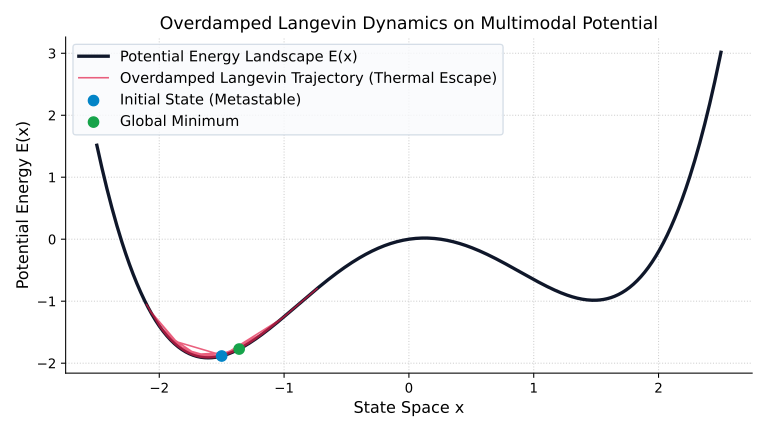
In molecular dynamics, biological fluids, and machine learning optimization, the relaxation time $\tau_r = m/\gamma$ is negligibly small compared to observation timescales. Setting $m \frac{dv}{dt} \to 0$ in the full Langevin equation with an external potential energy landscape $E(x)$:

$$0 = -\gamma \frac{dx}{dt} - \nabla E(x) + \eta(t)$$

Rearranging and defining mobility $\mu = 1/\gamma$:

$$\frac{dx}{dt} = -\mu \nabla E(x) + \mu \eta(t)$$

In standard stochastic calculus notation, setting units such that mobility $\mu = 1$ and thermal noise intensity $2 k_B T = 2T$, we obtain the Overdamped Langevin Stochastic Differential Equation (SDE):

$$dx_t = -\nabla E(x_t) dt + \sqrt{2T} \, dW_t$$

where $W_t$ is standard $d$-dimensional Brownian motion (Wiener process) satisfying $\mathbb{E}[dW_t] = 0$ and $\mathbb{E}[dW_t dW_t^T] = \mathbf{I} dt$.

Derivation of the Fokker-Planck Equation

Let $p(x, t)$ denote the probability density of finding the particle at position $x$ at time $t$. To derive the deterministic PDE governing the time evolution of $p(x, t)$, let $g(x): \mathbb{R}^d \to \mathbb{R}$ be an arbitrary smooth, compactly supported test function.

By Itô's Lemma, the differential of $g(x_t)$ along the trajectory of $dx_t = -\nabla E(x_t) dt + \sqrt{2T} dW_t$ is:

$$dg(x_t) = \nabla g(x_t)^T dx_t + \frac{1}{2} \operatorname{Tr}\left( \nabla^2 g(x_t) (dx_t)(dx_t)^T \right)$$

Since $(dW_t)(dW_t)^T = \mathbf{I} dt$ and $dt \cdot dW_t = 0$:

$$dg(x_t) = \left( -\nabla g(x_t)^T \nabla E(x_t) + T \Delta g(x_t) \right) dt + \sqrt{2T} \nabla g(x_t)^T dW_t$$

Taking the expectation $\mathbb{E}[\cdot]$ over all stochastic paths:

$$\frac{d}{dt} \mathbb{E}[g(x_t)] = \int_{\mathbb{R}^d} g(x) \frac{\partial p(x, t)}{\partial t} dx = \int_{\mathbb{R}^d} \left( -\nabla g(x)^T \nabla E(x) + T \Delta g(x) \right) p(x, t) dx$$

Using integration by parts (assuming $p(x,t)$ and its derivatives vanish at infinity):

1. For the drift term: $$-\int_{\mathbb{R}^d} (\nabla g \cdot \nabla E) p \, dx = \int_{\mathbb{R}^d} g(x) \nabla \cdot \left( p(x, t) \nabla E(x) \right) dx$$
2. For the diffusion term: $$T \int_{\mathbb{R}^d} (\Delta g) p \, dx = T \int_{\mathbb{R}^d} g(x) \Delta p(x, t) dx = T \int_{\mathbb{R}^d} g(x) \nabla^2 p(x, t) dx$$

Equating the integrals for all arbitrary test functions $g(x)$:

$$\frac{\partial p(x, t)}{\partial t} = \nabla \cdot \left( p(x, t) \nabla E(x) \right) + T \nabla^2 p(x, t)$$

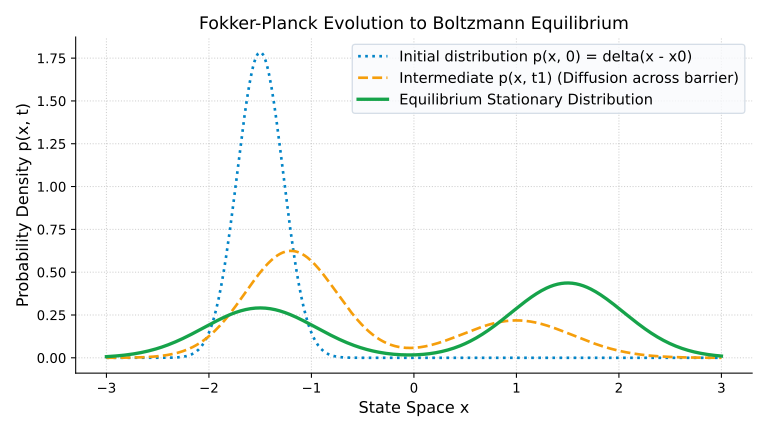
This is the Fokker-Planck (or Forward Kolmogorov) Equation.

Continuity Equation & Probability Current

We can rewrite the Fokker-Planck equation as a conservation law (continuity equation):

$$\frac{\partial p(x, t)}{\partial t} + \nabla \cdot J(x, t) = 0$$

where the Probability Current Density $J(x, t)$ is defined as:

$$J(x, t) = \underbrace{-p(x, t) \nabla E(x)}_{\text{Drift Current } J_{\mathrm{drift}}} - \underbrace{T \nabla p(x, t)}_{\text{Diffusion Current } J_{\mathrm{diff}}}$$

Convergence to Gibbs-Boltzmann Equilibrium

In the stationary state $\frac{\partial p(x, t)}{\partial t} = 0$, conservation requires $\nabla \cdot J_\infty(x) = 0$. Under thermal equilibrium, a stronger condition holds: Detailed Balance, which requires the probability current to vanish identically everywhere:

$$J_\infty(x) = -p_\infty(x) \nabla E(x) - T \nabla p_\infty(x) = 0$$

Dividing by $T p_\infty(x)$:

$$\frac{\nabla p_\infty(x)}{p_\infty(x)} = \nabla \log p_\infty(x) = -\frac{1}{T} \nabla E(x)$$

Integrating both sides with respect to $x$:

$$\log p_\infty(x) = -\frac{E(x)}{T} - \log Z \implies p_\infty(x) = \frac{1}{Z} e^{-\frac{E(x)}{T}}$$

where $Z = \int_{\mathbb{R}^d} e^{-E(x)/T} dx$ is the canonical partition function.

Relative Entropy as a Lyapunov Functional

How fast does $p(x, t)$ converge to $p_\infty(x)$? Let us consider the Kullback-Leibler divergence (Relative Entropy) as a Lyapunov function:

$$\mathcal{H}(t) = D_{\mathrm{KL}}(p(x, t) \,\|\, p_\infty(x)) = \int_{\mathbb{R}^d} p(x, t) \log \left( \frac{p(x, t)}{p_\infty(x)} \right) dx$$

Differentiating with respect to time $t$:

$$\begin{aligned} \frac{d}{dt} \mathcal{H}(t) &= \int \frac{\partial p}{\partial t} \left[ \log\left(\frac{p}{p_\infty}\right) + 1 \right] dx \\ &= \int (-\nabla \cdot J) \left[ \log\left(\frac{p}{p_\infty}\right) + 1 \right] dx \\ &= \int J(x, t) \cdot \nabla \log\left(\frac{p(x, t)}{p_\infty(x)}\right) dx \end{aligned}$$

Recalling $J(x, t) = -T p(x, t) \nabla \log\left(\frac{p(x, t)}{p_\infty(x)}\right)$:

$$\frac{d}{dt} D_{\mathrm{KL}}(p(x, t) \,\|\, p_\infty(x)) = -T \int_{\mathbb{R}^d} p(x, t) \left\| \nabla \log \frac{p(x, t)}{p_\infty(x)} \right\|^2 dx = -T \, \mathcal{I}(p(t) \,\|\, p_\infty) \le 0$$

where $\mathcal{I}(p \,\|\, p_\infty)$ is the Relative Fisher Information. Thus, $D_{\mathrm{KL}}$ decreases monotonically to zero.

Under the Logarithmic Sobolev Inequality (LSI) with constant $\rho > 0$:

$$D_{\mathrm{KL}}(p \,\|\, p_\infty) \le \frac{1}{2\rho} \mathcal{I}(p \,\|\, p_\infty) \implies \frac{d}{dt} D_{\mathrm{KL}}(t) \le -2\rho T D_{\mathrm{KL}}(t)$$

Integrating yields exponential convergence in entropy (exponential ergodicity):

$$D_{\mathrm{KL}}(p(x, t) \,\|\, p_\infty(x)) \le D_{\mathrm{KL}}(p(x, 0) \,\|\, p_\infty(x)) e^{-2\rho T t}$$

Discrete Algorithms: ULA and MALA

To sample from a target distribution $p(x) \propto e^{-E(x)}$ on a computer, we discretize the overdamped Langevin SDE with step size $\gamma_{\text{step}} > 0$:

1. Unadjusted Langevin Algorithm (ULA):

   $$x_{k+1} = x_k - \gamma_{\text{step}} \nabla E(x_k) + \sqrt{2T \gamma_{\text{step}}} \, z_k, \quad z_k \sim \mathcal{N}(0, \mathbf{I})$$

   Due to finite step size $\gamma_{\text{step}}$, the stationary distribution of ULA has an $\mathcal{O}(\gamma_{\text{step}})$ bias away from the true Gibbs target.

2. Metropolis-Adjusted Langevin Algorithm (MALA): Propose candidate $x'$ using ULA step, then accept/reject with Metropolis-Hastings probability:

   $$\alpha(x_k, x') = \min\left( 1, \frac{p(x') q(x_k | x')}{p(x_k) q(x' | x_k)} \right)$$

   where $q(x' | x_k) = \mathcal{N}\left( x'; x_k - \gamma_{\text{step}} \nabla E(x_k), 2T\gamma_{\text{step}} \mathbf{I} \right)$, restoring exact asymptotic convergence without step-size bias.

---

Denoising Diffusion Probabilistic Models (DDPM)

In 2015, Sohl-Dickstein et al. introduced deep generative modeling via non-equilibrium thermodynamics, which was later refined and popularized by Jonathan Ho, Ajay Jain, and Pieter Abbeel (NeurIPS 2020) into Denoising Diffusion Probabilistic Models (DDPM).

The Forward (Diffusion) Process

Let $x_0 \sim q(x_0)$ be a clean data sample from the target distribution. The forward process generates a sequence of latent variables $x_1, x_2, \dots, x_T$ by sequentially adding Gaussian noise according to a fixed variance schedule $\beta_1, \beta_2, \dots, \beta_T \in (0, 1)$:

$$q(x_{1:T} | x_0) = \prod_{t=1}^T q(x_t | x_{t-1}), \quad q(x_t | x_{t-1}) = \mathcal{N}\left( x_t; \sqrt{1 - \beta_t} x_{t-1}, \beta_t \mathbf{I} \right)$$

Closed-Form Marginal $q(x_t | x_0)$

Define $\alpha_t = 1 - \beta_t$ and the cumulative product $\bar{\alpha}_t = \prod_{s=1}^t \alpha_s$.

Using the recursive relation:

$$x_t = \sqrt{\alpha_t} x_{t-1} + \sqrt{1 - \alpha_t} \epsilon_{t-1}, \quad \epsilon_{t-1} \sim \mathcal{N}(0, \mathbf{I})$$

Substituting $x_{t-1} = \sqrt{\alpha_{t-1}} x_{t-2} + \sqrt{1 - \alpha_{t-1}} \epsilon_{t-2}$:

$$x_t = \sqrt{\alpha_t \alpha_{t-1}} x_{t-2} + \sqrt{\alpha_t(1 - \alpha_{t-1})} \epsilon_{t-2} + \sqrt{1 - \alpha_t} \epsilon_{t-1}$$

Because the sum of two independent Gaussians $\mathcal{N}(0, \sigma_1^2 \mathbf{I})$ and $\mathcal{N}(0, \sigma_2^2 \mathbf{I})$ is Gaussian with variance $(\sigma_1^2 + \sigma_2^2)\mathbf{I}$:

$$\alpha_t(1 - \alpha_{t-1}) + (1 - \alpha_t) = 1 - \alpha_t \alpha_{t-1}$$

By induction across all $t$ steps:

$$q(x_t | x_0) = \mathcal{N}\left( x_t; \sqrt{\bar{\alpha}_t} x_0, (1 - \bar{\alpha}_t) \mathbf{I} \right)$$

Hence, we can sample $x_t$ at any arbitrary timestep $t$ directly in closed form:

$$x_t = \sqrt{\bar{\alpha}_t} x_0 + \sqrt{1 - \bar{\alpha}_t} \epsilon, \quad \epsilon \sim \mathcal{N}(0, \mathbf{I})$$

The Reverse (Generative) Process & The ELBO

The generative model is defined as a Markov chain with learned Gaussian transitions running backward in time from $p(x_T) = \mathcal{N}(x_T; 0, \mathbf{I})$:

$$p_\theta(x_{0:T}) = p(x_T) \prod_{t=1}^T p_\theta(x_{t-1} | x_t), \quad p_\theta(x_{t-1} | x_t) = \mathcal{N}\left( x_{t-1}; \mu_\theta(x_t, t), \Sigma_\theta(x_t, t) \right)$$

To train $\theta$, we maximize the marginal log-likelihood $\mathbb{E}_{q(x_0)}[\log p_\theta(x_0)]$ via the Variational Lower Bound (ELBO):

$$\begin{aligned} \log p_\theta(x_0) &\ge \mathbb{E}_{q(x_{1:T} | x_0)} \left[ \log \frac{p_\theta(x_{0:T})}{q(x_{1:T} | x_0)} \right] \\ &= \mathbb{E}_q \left[ \log \frac{p(x_T) \prod_{t=1}^T p_\theta(x_{t-1} | x_t)}{\prod_{t=1}^T q(x_t | x_{t-1})} \right] \end{aligned}$$

Using Bayes' rule on the forward transitions $q(x_t | x_{t-1}) = \frac{q(x_{t-1} | x_t, x_0) q(x_t | x_0)}{q(x_{t-1} | x_0)}$:

$$\begin{aligned} \frac{p_\theta(x_{0:T})}{q(x_{1:T} | x_0)} &= \frac{p(x_T) p_\theta(x_0 | x_1) \prod_{t=2}^T p_\theta(x_{t-1} | x_t)}{q(x_1 | x_0) \prod_{t=2}^T q(x_{t-1} | x_t, x_0) \frac{q(x_t | x_0)}{q(x_{t-1} | x_0)}} \\ &= \frac{p(x_T)}{q(x_T | x_0)} \cdot p_\theta(x_0 | x_1) \cdot \prod_{t=2}^T \frac{p_\theta(x_{t-1} | x_t)}{q(x_{t-1} | x_t, x_0)} \end{aligned}$$

Taking the logarithm and expectation yields the canonical three-part decomposition:

$$\mathcal{L}_{\mathrm{VLB}} = \mathbb{E}_q \left[ \underbrace{D_{\mathrm{KL}}(q(x_T | x_0) \,\|\, p(x_T))}_{L_T \text{ (Prior Matching)}} + \sum_{t=2}^T \underbrace{D_{\mathrm{KL}}(q(x_{t-1} | x_t, x_0) \,\|\, p_\theta(x_{t-1} | x_t))}_{L_{t-1} \text{ (Denoising Matching)}} - \underbrace{\log p_\theta(x_0 | x_1)}_{L_0 \text{ (Reconstruction)}} \right]$$

Tractable Posterior $q(x_{t-1} | x_t, x_0)$

Using Bayes' rule for Gaussians, the forward posterior conditioned on $x_0$ is analytically tractable:

$$q(x_{t-1} | x_t, x_0) = \frac{q(x_t | x_{t-1}, x_0) q(x_{t-1} | x_0)}{q(x_t | x_0)} = \mathcal{N}\left( x_{t-1}; \tilde{\mu}_t(x_t, x_0), \tilde{\beta}_t \mathbf{I} \right)$$

Expanding exponents:

$$\begin{aligned} q(x_{t-1} | x_t, x_0) &\propto \exp\left( -\frac{1}{2} \left[ \frac{\|x_t - \sqrt{\alpha_t} x_{t-1}\|^2}{\beta_t} + \frac{\|x_{t-1} - \sqrt{\bar{\alpha}_{t-1}} x_0\|^2}{1 - \bar{\alpha}_{t-1}} - \frac{\|x_t - \sqrt{\bar{\alpha}_t} x_0\|^2}{1 - \bar{\alpha}_t} \right] \right) \\ &= \exp\left( -\frac{1}{2} \left[ x_{t-1}^T \left( \frac{\alpha_t}{\beta_t} + \frac{1}{1 - \bar{\alpha}_{t-1}} \right) x_{t-1} - 2 x_{t-1}^T \left( \frac{\sqrt{\alpha_t}}{\beta_t} x_t + \frac{\sqrt{\bar{\alpha}_{t-1}}}{1 - \bar{\alpha}_{t-1}} x_0 \right) + C(x_t, x_0) \right] \right) \end{aligned}$$

Matching precision (inverse variance) $\tilde{\beta}_t^{-1}$:

$$\tilde{\beta}_t^{-1} = \frac{\alpha_t(1 - \bar{\alpha}_{t-1}) + \beta_t}{\beta_t(1 - \bar{\alpha}_{t-1})} = \frac{1 - \bar{\alpha}_t}{\beta_t(1 - \bar{\alpha}_{t-1})} \implies \tilde{\beta}_t = \frac{1 - \bar{\alpha}_{t-1}}{1 - \bar{\alpha}_t} \beta_t$$

Matching mean $\tilde{\mu}_t(x_t, x_0)$:

$$\tilde{\mu}_t(x_t, x_0) = \tilde{\beta}_t \left( \frac{\sqrt{\alpha_t}}{\beta_t} x_t + \frac{\sqrt{\bar{\alpha}_{t-1}}}{1 - \bar{\alpha}_{t-1}} x_0 \right) = \frac{\sqrt{\alpha_t}(1 - \bar{\alpha}_{t-1})}{1 - \bar{\alpha}_t} x_t + \frac{\sqrt{\bar{\alpha}_{t-1}}\beta_t}{1 - \bar{\alpha}_t} x_0$$

The $\epsilon$-Parameterization & Connection to Score Matching

Since $x_t = \sqrt{\bar{\alpha}_t} x_0 + \sqrt{1 - \bar{\alpha}_t} \epsilon$, we express $x_0$ in terms of $x_t$ and noise $\epsilon$:

$$x_0 = \frac{x_t - \sqrt{1 - \bar{\alpha}_t} \epsilon}{\sqrt{\bar{\alpha}_t}}$$

Substituting this into $\tilde{\mu}_t(x_t, x_0)$:

$$\begin{aligned} \tilde{\mu}_t(x_t, x_0) &= \frac{\sqrt{\alpha_t}(1 - \bar{\alpha}_{t-1})}{1 - \bar{\alpha}_t} x_t + \frac{\sqrt{\bar{\alpha}_{t-1}}\beta_t}{1 - \bar{\alpha}_t} \left( \frac{x_t - \sqrt{1 - \bar{\alpha}_t} \epsilon}{\sqrt{\bar{\alpha}_t}} \right) \\ &= \frac{1}{\sqrt{\alpha_t}} \left( x_t - \frac{\beta_t}{\sqrt{1 - \bar{\alpha}_t}} \epsilon \right) \end{aligned}$$

Ho et al. therefore parameterized the neural network $\mu_\theta(x_t, t)$ to predict the injected noise $\epsilon_\theta(x_t, t)$:

$$\mu_\theta(x_t, t) = \frac{1}{\sqrt{\alpha_t}} \left( x_t - \frac{\beta_t}{\sqrt{1 - \bar{\alpha}_t}} \epsilon_\theta(x_t, t) \right)$$

The KL divergence between two Gaussians with identical variance $\sigma_t^2 \mathbf{I}$ simplifies to:

$$L_{t-1} = \mathbb{E}_q \left[ \frac{1}{2\sigma_t^2} \|\tilde{\mu}_t(x_t, x_0) - \mu_\theta(x_t, t)\|^2 \right] = \mathbb{E}_{x_0, \epsilon} \left[ \frac{\beta_t^2}{2\sigma_t^2 \alpha_t (1 - \bar{\alpha}_t)} \|\epsilon - \epsilon_\theta(\sqrt{\bar{\alpha}_t} x_0 + \sqrt{1 - \bar{\alpha}_t}\epsilon, t)\|^2 \right]$$

Dropping the weighting factor yields the celebrated DDPM Simplified Loss Function:

$$\mathcal{L}_{\mathrm{simple}}(\theta) = \mathbb{E}_{t \sim \mathcal{U}(1, T), x_0 \sim q(x_0), \epsilon \sim \mathcal{N}(0, \mathbf{I})} \left[ \left\| \epsilon - \epsilon_\theta\left( \sqrt{\bar{\alpha}_t} x_0 + \sqrt{1 - \bar{\alpha}_t} \epsilon, \, t \right) \right\|^2 \right]$$

---

Score-Based Generative Modeling through SDEs (Score-SDE)

In 2021, Yang Song, Jascha Sohl-Dickstein, Diederik P. Kingma, Abhishek Kumar, Stefano Ermon, and Ben Poole unified DDPMs and Score-Based Generative Networks under the continuous-time framework of Stochastic Differential Equations (SDEs).

The Forward SDE Framework

In the continuous-time limit ($T \to \infty, \Delta t \to 0$), the forward diffusion process is described by an Itô SDE:

$$dx = f(x, t) dt + g(t) dW_t, \quad t \in [0, T]$$

where $f(x, t) \in \mathbb{R}^d$ is the vector-valued drift coefficient, $g(t) \in \mathbb{R}$ is the scalar diffusion coefficient, and $W_t \in \mathbb{R}^d$ is standard Brownian motion.

Three prominent continuous SDE families exist in the literature:

1. Variance Preserving SDE (VP-SDE) (Continuous DDPM): $$f(x, t) = -\frac{1}{2} \beta(t) x, \quad g(t) = \sqrt{\beta(t)}$$
2. Variance Exploding SDE (VE-SDE) (Continuous NCSN / Score Matching): $$f(x, t) = 0, \quad g(t) = \sqrt{\frac{d[\sigma^2(t)]}{dt}}$$
3. sub-VP SDE: $$f(x, t) = -\frac{1}{2} \beta(t) x, \quad g(t) = \sqrt{\beta(t) \left( 1 - e^{-2 \int_0^t \beta(s) ds} \right)}$$

Anderson's Reverse-Time SDE Theorem

In a foundational 1982 paper, Brian D. O. Anderson proved that any forward diffusion process governed by Itô SDE $dx = f(x, t) dt + g(t) dW_t$ possesses an exact reverse-time stochastic trajectory running backward from $t = T$ to $t = 0$.

Complete Mathematical Proof via Fokker-Planck Equivalence

We now provide the rigorous derivation by proving that the forward and reverse SDEs generate identical marginal densities $p_t(x)$ at every instant $t \in [0, T]$.

Step 1: Forward Fokker-Planck Equation. The forward SDE $dx = f(x, t) dt + g(t) dW_t$ has probability current $J_f(x, t) = p_t(x) f(x, t) - \frac{1}{2} g(t)^2 \nabla_x p_t(x)$. Its Fokker-Planck equation is:

$$\frac{\partial p_t(x)}{\partial t} = -\nabla_x \cdot \left[ p_t(x) f(x, t) \right] + \frac{1}{2} g(t)^2 \nabla_x^2 p_t(x)$$

Step 2: Reverse SDE Ansatz. Assume a general reverse-time SDE running backward with drift $\tilde{f}(x, t)$ and identical diffusion coefficient $g(t)$:

$$dx = \tilde{f}(x, t) dt + g(t) d\bar{W}_t$$

Reversing time via substitution $\tau = -t$, the time derivative satisfies $\frac{\partial}{\partial \tau} = -\frac{\partial}{\partial t}$. The Fokker-Planck equation for this reverse process running backward must satisfy:

$$-\frac{\partial p_t(x)}{\partial t} = -\nabla_x \cdot \left[ p_t(x) \tilde{f}(x, t) \right] + \frac{1}{2} g(t)^2 \nabla_x^2 p_t(x)$$

Rearranging:

$$\frac{\partial p_t(x)}{\partial t} = \nabla_x \cdot \left[ p_t(x) \tilde{f}(x, t) \right] - \frac{1}{2} g(t)^2 \nabla_x^2 p_t(x)$$

Step 3: Equating Forward and Reverse Fokker-Planck Equations. For the reverse process to have the exact same marginals $p_t(x)$ as the forward process, the two time-derivative expressions must match:

$$-\nabla_x \cdot \left[ p_t(x) f(x, t) \right] + \frac{1}{2} g(t)^2 \nabla_x^2 p_t(x) = \nabla_x \cdot \left[ p_t(x) \tilde{f}(x, t) \right] - \frac{1}{2} g(t)^2 \nabla_x^2 p_t(x)$$

Combining terms:

$$\nabla_x \cdot \left[ p_t(x) \left( \tilde{f}(x, t) + f(x, t) \right) \right] = g(t)^2 \nabla_x^2 p_t(x)$$

Using the identity $\nabla_x^2 p_t(x) = \nabla_x \cdot \left( \nabla_x p_t(x) \right) = \nabla_x \cdot \left( p_t(x) \nabla_x \log p_t(x) \right)$:

$$\nabla_x \cdot \left[ p_t(x) \left( \tilde{f}(x, t) + f(x, t) \right) \right] = \nabla_x \cdot \left[ p_t(x) \left( g(t)^2 \nabla_x \log p_t(x) \right) \right]$$

Equating the vector fields inside the divergence (under zero boundary conditions at infinity):

$$p_t(x) \left( \tilde{f}(x, t) + f(x, t) \right) = p_t(x) \left( g(t)^2 \nabla_x \log p_t(x) \right)$$

Dividing by $p_t(x) > 0$:

$$\tilde{f}(x, t) = -f(x, t) + g(t)^2 \nabla_x \log p_t(x)$$

Since time flows backward ($dt < 0$), the drift term appearing in $dx = \tilde{f}_{\text{eff}}(x, t) dt$ is:

$$dx = \left[ f(x, t) - g(t)^2 \nabla_x \log p_t(x) \right] dt + g(t) d\bar{W}_t \quad \blacksquare$$

The Probability Flow ODE

Remarkably, Song et al. (2021) demonstrated that there exists a completely deterministic ordinary differential equation (ODE) whose trajectory shares the exact same marginal probability density $p_t(x)$ as the stochastic SDE for all $t \in [0, T]$:

$$\frac{dx}{dt} = f(x, t) - \frac{1}{2} g(t)^2 \nabla_x \log p_t(x)$$

Exact Log-Likelihood via the Instantaneous Change of Variables

For any sample $x_0$, we can compute its exact likelihood under the model by integrating the divergence of the ODE vector field $v(x, t) = f(x, t) - \frac{1}{2} g(t)^2 s_\theta(x, t)$ using the continuous change-of-variables formula:

$$\log p_0(x_0) = \log p_T(x_T) + \int_0^T \nabla_x \cdot \left[ f(x(t), t) - \frac{1}{2} g(t)^2 s_\theta(x(t), t) \right] dt$$

The high-dimensional trace/divergence $\nabla_x \cdot v(x, t) = \operatorname{Tr}(\nabla_x v(x, t))$ is computed efficiently via the Hutchinson Trace Estimator:

$$\operatorname{Tr}(\nabla_x v(x, t)) = \mathbb{E}_{\epsilon \sim \mathcal{N}(0, \mathbf{I})} \left[ \epsilon^T \nabla_x v(x, t) \epsilon \right]$$

which requires only a single vector-Jacobian product (VJP) via reverse-mode automatic differentiation.

Score Matching Objectives

To train a neural network $s_\theta(x, t)$ to approximate $\nabla_x \log p_t(x)$ without knowing the intractable normalizing partition function of $p_t(x)$, we use Score Matching.

1. Explicit Score Matching (ESM)

The ideal Fisher divergence objective:

$$\mathcal{J}_{\mathrm{ESM}}(\theta) = \frac{1}{2} \mathbb{E}_{p_{\mathrm{data}}(x)} \left[ \left\| s_\theta(x) - \nabla_x \log p_{\mathrm{data}}(x) \right\|^2 \right]$$

This is intractable because the ground truth score $\nabla_x \log p_{\mathrm{data}}(x)$ is unknown.

2. Implicit Score Matching (ISM - Aapo Hyvärinen, 2005)

Expanding the square in ESM:

$$\mathcal{J}_{\mathrm{ESM}}(\theta) = \mathbb{E}_{p(x)} \left[ \frac{1}{2} \|s_\theta(x)\|^2 - s_\theta(x) \cdot \nabla_x \log p(x) \right] + \text{const}$$

Applying integration by parts on the cross-term:

$$\int_{\mathbb{R}^d} p(x) s_\theta(x) \cdot \frac{\nabla p(x)}{p(x)} dx = \int_{\mathbb{R}^d} s_\theta(x) \cdot \nabla p(x) dx = -\int_{\mathbb{R}^d} p(x) \nabla \cdot s_\theta(x) dx = -\mathbb{E}_{p(x)}[\operatorname{Tr}(\nabla_x s_\theta(x))]$$

This yields the Implicit Score Matching Objective:

$$\mathcal{J}_{\mathrm{ISM}}(\theta) = \mathbb{E}_{p_{\mathrm{data}}(x)} \left[ \operatorname{Tr}\left( \nabla_x s_\theta(x) \right) + \frac{1}{2} \|s_\theta(x)\|^2 \right]$$

3. Denoising Score Matching (DSM - Pascal Vincent, 2011)

Perturb data $x_0 \sim q(x_0)$ with a known transition kernel $q(x_t | x_0) = \mathcal{N}(x_t; \mu(x_0, t), \sigma^2(t) \mathbf{I})$. Vincent proved that:

$$\nabla_{x_t} \log q(x_t) = \mathbb{E}_{q(x_0 | x_t)} \left[ \nabla_{x_t} \log q(x_t | x_0) \right]$$

The tractable objective optimizes score prediction against the analytic conditional kernel:

$$\mathcal{J}_{\mathrm{DSM}}(\theta) = \mathbb{E}_{t \sim \mathcal{U}(0, T), x_0 \sim q(x_0), x_t \sim q(x_t | x_0)} \left[ \lambda(t) \left\| s_\theta(x_t, t) - \nabla_{x_t} \log q(x_t | x_0) \right\|^2 \right]$$

Since $\nabla_{x_t} \log q(x_t | x_0) = -\frac{x_t - \mu(x_0, t)}{\sigma^2(t)} = -\frac{\epsilon}{\sigma(t)}$, DSM reduces exactly to the noise regression loss used in DDPM.

Predictor-Corrector (PC) Sampling

Song et al. introduced Predictor-Corrector (PC) Samplers, which combine numerical integration of the reverse SDE with intermediate Langevin MCMC corrections:

The Corrector uses the learned score $s_\theta(x_t, t)$ to actively suppress accumulated numerical drift and discretization error, guaranteeing high sampling fidelity.

---

Discrete Diffusion Models for Language & Symbolic Spaces

While continuous diffusion operates in Euclidean spaces $\mathbb{R}^d$, language models, symbolic mathematics, and biological sequences exist on discrete vocabularies $\mathcal{V} = \{1, 2, \dots, V\}^N$. On a discrete lattice, the gradient operator $\nabla_x \log p(x)$ is undefined.

Paradigm 1: Continuous Embedding Diffusion (Diffusion-LM)

In Diffusion-LM (Li et al., 2022), discrete token sequences $w = (w_1, \dots, w_N)$ are mapped into continuous embedding space $x_0 = \operatorname{Embed}(w) \in \mathbb{R}^{N \times d}$. Gaussian diffusion is performed in continuous space, and at step $t=0$, tokens are recovered via categorical rounding:

$$p_\theta(w | x_0) = \prod_{i=1}^N \operatorname{softmax}\left( E(w_i)^T x_0^{(i)} \right)$$

Fundamental Bottleneck: Continuous embeddings suffer from rounding collapse and out-of-vocabulary drift during intermediate timesteps, where continuous latents wander into regions of embedding space that do not correspond to any valid grammatical token sequence.

Paradigm 2: Continuous-Time Markov Chains & Score Entropy (SEDD)

To overcome the embedding bottleneck, Lou et al. (ICML 2024) formulated Score Entropy Discrete Diffusion (SEDD) directly on the discrete state space $\mathcal{V}^N$ using Continuous-Time Markov Chains (CTMC).

The Master Equation of Discrete Diffusion

Let $x_t \in \mathcal{V}^N$ evolve according to a transition rate matrix $Q_t \in \mathbb{R}^{V \times V}$, where $Q_t(x, y) \ge 0$ ($x \neq y$) is the instantaneous jump rate from state $x$ to state $y$, with diagonal $Q_t(x, x) = -\sum_{y \neq x} Q_t(x, y)$.

The probability distribution $p_t(x)$ obeys the continuous-time Master Equation:

$$\frac{d p_t(x)}{dt} = \sum_{y \in \mathcal{V}} p_t(y) Q_t(y, x) = \sum_{y \neq x} \left[ p_t(y) Q_t(y, x) - p_t(x) Q_t(x, y) \right]$$

Time-Reversal of Discrete CTMC (Kelly's Lemma)

By Kolmogorov's time-reversal theorem for jump processes, the reverse-time process running from $t = T$ back to $t = 0$ is itself a continuous-time Markov chain with reverse transition rate matrix $\bar{Q}_t(x, y)$:

$$\bar{Q}_t(x, y) = Q_t(y, x) \frac{p_t(y)}{p_t(x)}$$

Score Entropy Loss

SEDD replaces Euclidean score matching with the Score Entropy Objective:

$$\mathcal{L}_{\mathrm{SEDD}}(\theta) = \mathbb{E}_{t, x_0, x_t} \left[ \sum_{y \neq x_t} Q_t(x_t, y) \left( s_\theta(x_t, y, t) - \frac{q(y | x_0)}{q(x_t | x_0)} \log s_\theta(x_t, y, t) \right) \right]$$

Minimizing $\mathcal{L}_{\mathrm{SEDD}}$ forces the neural network $s_\theta(x_t, y, t)$ to converge to the exact time-reversal transition rates $\bar{Q}_t(x_t, y)$, enabling rigorous discrete generation without continuous relaxation.

Paradigm 3: Masking-Based Discrete Diffusion & LLaDA 8B

In late 2024 and 2025, Large Language Diffusion Models underwent a major breakthrough with LLaDA (Large Language Diffusion with Masking) (Nie et al., NeurIPS 2025 / 2024), scaling discrete diffusion to an 8-billion parameter foundational model competitive with LLaMA3.

The Absorbing State (Masking) Kernel

Instead of uniform substitution across the vocabulary $\mathcal{V}$, LLaDA employs an absorbing state transition with a dedicated [MASK] token:

$$q(x_t^i | x_0^i) = \begin{cases} x_0^i & \text{with probability } \alpha_t \\ \text{[MASK]} & \text{with probability } 1 - \alpha_t \end{cases}$$

where $\alpha_t = 1 - t/T$ is a monotonic unmasking schedule ($t \in [0, T]$).

Training Objective

At training time, given a sequence $x_0 = (x_0^1, \dots, x_0^N)$, a time $t \sim \mathcal{U}(0, T)$ is sampled, masking a subset of tokens $\mathcal{M}_t \subseteq \{1, \dots, N\}$. The Transformer network $p_\theta(x_0^i | x_t)$ is trained via bidirectional cross-entropy loss only on the masked positions:

$$\mathcal{L}_{\mathrm{LLaDA}}(\theta) = \mathbb{E}_{t, x_0, \mathcal{M}_t} \left[ \sum_{i \in \mathcal{M}_t} -\log p_\theta\left( x_0^i \,\Big|\, x_t \right) \right]$$

Re-masking and Semi-Autoregressive Sampling

During inference, LLaDA generates an entire document non-autoregressively or semi-autoregressively via iterative unmasking:

def llada_reverse_generation(sequence_length, total_steps, temperature):
    """
    LLaDA Masked Diffusion Reverse Sampling Algorithm
    """
    # 1. Initialize full masked sequence
    x = [MASK] * sequence_length
    
    for k in range(total_steps, 0, -1):
        # Predict token probabilities for masked positions
        p_theta = model.predict_logits(x) / temperature
        sampled_tokens = categorical_sample(p_theta)
        
        # Calculate confidence scores
        confidence = compute_confidence(p_theta, sampled_tokens)
        
        # Determine number of tokens to unmask at this step
        num_unmasked = schedule(k, total_steps, sequence_length)
        top_indices = get_top_k_indices(confidence, k=num_unmasked)
        
        for idx in top_indices:
            x[idx] = sampled_tokens[idx]
            
    return x

Comparative Analysis: Autoregressive LLMs vs. Discrete Diffusion LLMs

---

Thermodynamic Entropy Production & The Direction of Time

We conclude by tying all generative diffusion frameworks back to fundamental Non-Equilibrium Thermodynamics.

$\Delta S_{\text{tot}} = \ln \frac{\mathcal{P}[x(t)]}{\mathcal{P}^{\text{rev}}[x(T-t)]} = \Delta S_{\text{sys}} + \Delta S_{\text{medium}} \ge 0$

Consider the path probability measure $\mathcal{P}[x(t)]_{t=0}^T$ of the forward diffusion process and the time-reversed path measure $\mathcal{P}_R[\bar{x}(t)]_{t=0}^T$. By the Crooks Fluctuation Theorem and the Second Law of Thermodynamics, the total entropy production along the stochastic trajectory is:

$$\Delta S_{\mathrm{tot}} = D_{\mathrm{KL}}\left( \mathcal{P}[x(t)] \,\|\, \mathcal{P}_R[\bar{x}(t)] \right) \ge 0$$

Expanding the path integral under the forward SDE $dx = f dt + g dW_t$ and parameterized reverse model $dx = [f - g^2 s_\theta] dt + g d\bar{W}_t$ via Girsanov's Theorem:

$$\Delta S_{\mathrm{tot}} = \frac{1}{2} \int_0^T g(t)^2 \, \mathbb{E}_{p_t(x)} \left[ \left\| s_\theta(x, t) - \nabla_x \log p_t(x) \right\|^2 \right] dt = \int_0^T \mathcal{J}_{\mathrm{ESM}}(\theta, t) \, dt$$

[!IMPORTANT] The Thermodynamic Nature of Diffusion Training: Minimizing the score-matching loss $\mathcal{J}_{\mathrm{ESM}}(\theta)$ is mathematically identical to minimizing the total thermodynamic entropy production of the time-reversal process.

When the neural score network achieves zero loss ($s_\theta(x, t) = \nabla_x \log p_t(x)$), total entropy production vanishes ($\Delta S_{\mathrm{tot}} = 0$), meaning the artificial generative process operates as an ideal, microscopically reversible thermodynamic engine running backwards in time.

---

Summary of Key Theoretical Results

---

References & Foundational Literature

1. Langevin, P. (1908). Sur la théorie du mouvement brownien. C. R. Acad. Sci. (Paris), 146, 530–533.
2. Einstein, A. (1905). Über die von der molekularkinetischen Theorie der Wärme geforderte Bewegung von in ruhenden Flüssigkeiten suspendierten Teilchen. Annalen der Physik, 322(8), 549–560.
3. Anderson, B. D. O. (1982). Reverse-time diffusion equation models. Stochastic Processes and their Applications, 12(3), 313–326.
4. Hyvärinen, A. (2005). Estimation of non-normalized statistical models by score matching. Journal of Machine Learning Research, 6(4), 695–709.
5. Vincent, P. (2011). A connection between score matching and denoising autoencoders. Neural Computation, 23(7), 1661–1674.
6. Sohl-Dickstein, J., Weiss, E., Khanshali, N., & Sompolinsky, H. (2015). Deep unsupervised learning using nonequilibrium thermodynamics. ICML 2015.
7. Song, Y., & Ermon, S. (2019). Generative modeling by estimating gradients of the data distribution. NeurIPS 2019.
8. Ho, J., Jain, A., & Abbeel, P. (2020). Denoising diffusion probabilistic models. NeurIPS 2020.
9. Song, Y., Sohl-Dickstein, J., Kingma, D. P., Kumar, A., Ermon, S., & Poole, B. (2021). Score-based generative modeling through stochastic differential equations. ICLR 2021.
10. Li, X. L., Thickstun, J., Gulrajani, I., Liang, P., & Hashimoto, T. B. (2022). Diffusion-LM improves controllable text generation. NeurIPS 2022.
11. Lou, A., Meng, C., & Ermon, S. (2024). Discrete diffusion modeling by estimating the score of the continuous-time Markov chain. ICML 2024.
12. Nie, S., et al. (2025). Large Language Diffusion Models (LLaDA). NeurIPS 2025 / arXiv:2410.02416.