Large Numbers, Self-Averaging & Infinite-Width Neural Networks

Why does statistical physics make exact, deterministic predictions about macroscopic systems composed of $10^{23}$ chaotic particles? And why do modern deep neural networks with billions of randomly initialized parameters converge reliably, behave deterministically in the wide limit, and generalize predictably across unseen data?

The answer to both questions lies in the mathematics of large numbers, concentration of measure, and self-averaging. In physical systems, microscopic fluctuations cancel out, giving rise to sharp thermodynamic laws. In deep learning, sending the layer width $N \to \infty$ simplifies intractable non-convex optimization into linear dynamics over deterministic kernel regimes: the Neural Network Gaussian Process (NNGP) and the Neural Tangent Kernel (NTK).

When finite width $N < \infty$ is restored, the system develops fluctuations and interactions that can be systematically computed via $1/N$ perturbative expansions (Feynman diagrams in statistical field theory), shedding light on representation learning and finite-sample SGD noise.

---

1. Microscopic Multiplicities, Binomial Distribution & Stirling's Asymptotics

To understand how deterministic macroscopic behavior emerges from stochastic microscopic degrees of freedom, we begin with the simplest combinatorial system: non-interacting binary degrees of freedom (e.g., non-interacting gas molecules in a partitioned volume or uncoupled Ising spins $\sigma_i \in \{-1, +1\}$).

1.1 Multiplicity and the Binomial Distribution

Consider $N$ independent particles placed in a container divided into two equal halves. Each particle has probability $p = 1/2$ of occupying the left half and $1-p = 1/2$ of occupying the right half. The total number of microstates is $\Omega_{\mathrm{total}} = 2^N$.

The number of distinct configurations (microstates) where exactly $m$ particles reside in the left half is given by the binomial coefficient:

$$\Omega(m; N) = \binom{N}{m} = \frac{N!}{m!\,(N-m)!}$$

The probability $P(m; N)$ of observing macrostate $m$ under the postulate of equal a priori probabilities is:

$$P(m; N) = \binom{N}{m} p^m (1-p)^{N-m} = \frac{1}{2^N} \frac{N!}{m!\,(N-m)!}$$

For small $N$, $P(m; N)$ is spread broadly across possible values of $m$. But when $N$ is on the order of Avogadro's number ($N \approx 10^{23}$), observing even a $0.0001\%$ relative deviation from the mean $m^* = N/2$ becomes astronomically impossible.

---

1.2 Step-by-Step Derivation of Stirling's Approximation via Laplace's Method

To analyze the behavior of $N!$ as $N \to \infty$, we express the factorial using Euler's Gamma function:

$$N! = \Gamma(N+1) = \int_0^\infty t^N e^{-t} \, dt = \int_0^\infty e^{N \ln t - t} \, dt$$

Let $h(t) = N \ln t - t$. To apply Laplace's method (the saddle-point approximation), we locate the maximum $t_0$ of $h(t)$:

$$h'(t) = \frac{N}{t} - 1 = 0 \implies t_0 = N$$

The second derivative at the saddle point is:

$$h''(t_0) = -\frac{N}{t_0^2} = -\frac{1}{N} < 0$$

Now perform a change of variables $t = N(1 + u)$, so that $dt = N \, du$:

$$\begin{aligned} h(t) &= N \ln(N(1+u)) - N(1+u) \\ &= N \ln N - N + N \left[ \ln(1+u) - u \right] \end{aligned}$$

Using the Taylor series expansion $\ln(1+u) = u - \frac{u^2}{2} + \frac{u^3}{3} - \mathcal{O}(u^4)$:

$$\ln(1+u) - u = -\frac{u^2}{2} + \frac{u^3}{3} - \frac{u^4}{4} + \dots$$

Substituting this into the integral:

$$\begin{aligned} N! &= \int_{-1}^\infty \exp\left( N \ln N - N - \frac{N u^2}{2} + \frac{N u^3}{3} - \dots \right) N \, du \\ &= N^{N+1} e^{-N} \int_{-1}^\infty e^{-\frac{N u^2}{2}} \exp\left( \frac{N u^3}{3} - \frac{N u^4}{4} + \dots \right) du \end{aligned}$$

Let $v = \sqrt{N} u$, so $du = \frac{dv}{\sqrt{N}}$:

$$N! = N^{N+1} e^{-N} \frac{1}{\sqrt{N}} \int_{-\sqrt{N}}^\infty e^{-v^2 / 2} \exp\left( \frac{v^3}{3\sqrt{N}} - \frac{v^4}{4N} + \dots \right) dv$$

Expanding the exponential perturbatively:

$$\exp\left( \frac{v^3}{3\sqrt{N}} - \frac{v^4}{4N} \right) = 1 + \frac{v^3}{3\sqrt{N}} + \left( \frac{v^6}{18N} - \frac{v^4}{4N} \right) + \mathcal{O}(N^{-3/2})$$

Using Gaussian moments $\int_{-\infty}^\infty e^{-v^2/2} dv = \sqrt{2\pi}$, $\int_{-\infty}^\infty v^3 e^{-v^2/2} dv = 0$ (odd symmetry), $\int_{-\infty}^\infty v^4 e^{-v^2/2} dv = 3\sqrt{2\pi}$, and $\int_{-\infty}^\infty v^6 e^{-v^2/2} dv = 15\sqrt{2\pi}$:

$$\begin{aligned} \int_{-\infty}^\infty e^{-v^2/2} \left[ 1 + \frac{1}{N}\left( \frac{v^6}{18} - \frac{v^4}{4} \right) \right] dv &= \sqrt{2\pi} \left[ 1 + \frac{1}{N}\left( \frac{15}{18} - \frac{3}{4} \right) \right] \\ &= \sqrt{2\pi} \left[ 1 + \frac{1}{12N} + \mathcal{O}(N^{-2}) \right] \end{aligned}$$

Thus, we obtain the full asymptotic Stirling series:

---

1.3 Asymptotics of the Binomial Distribution & Gaussian Emergence

We now evaluate the binomial log-probability $\ln P(m; N)$ for $m = N p + \delta m$, where $\delta m = \mathcal{O}(\sqrt{N})$ represents microscopic fluctuations around the expected mean.

Using $\ln N! \approx N \ln N - N + \frac{1}{2}\ln(2\pi N)$:

$$\begin{aligned} \ln P(m; N) &= \ln N! - \ln m! - \ln(N-m)! + m \ln p + (N-m) \ln(1-p) \\ &\approx N \ln N - N + \frac{1}{2}\ln(2\pi N) \\ &\quad - \left[ m \ln m - m + \frac{1}{2}\ln(2\pi m) \right] \\ &\quad - \left[ (N-m) \ln(N-m) - (N-m) + \frac{1}{2}\ln(2\pi(N-m)) \right] \\ &\quad + m \ln p + (N-m) \ln(1-p) \end{aligned}$$

Let $x = m/N = p + \frac{\delta m}{N} = p + \epsilon$, where $\epsilon = \frac{\delta m}{N} = \mathcal{O}(N^{-1/2})$. Expanding the terms:

$$\begin{aligned} -m \ln m - (N-m)\ln(N-m) + m \ln p + (N-m)\ln(1-p) &= -N \left[ x \ln\frac{x}{p} + (1-x)\ln\frac{1-x}{1-p} \right] \\ &= -N D_{\mathrm{KL}}(x \,\|\, p) \end{aligned}$$

Expanding the Kullback-Leibler divergence $D_{\mathrm{KL}}(p + \epsilon \,\|\, p)$ around $\epsilon = 0$:

$$D_{\mathrm{KL}}(p+\epsilon \,\|\, p) = \left. D_{\mathrm{KL}} \right|_{\epsilon=0} + \left. \epsilon \frac{\partial D_{\mathrm{KL}}}{\partial \epsilon} \right|_{\epsilon=0} + \left. \frac{\epsilon^2}{2} \frac{\partial^2 D_{\mathrm{KL}}}{\partial \epsilon^2} \right|_{\epsilon=0} + \mathcal{O}(\epsilon^3)$$

The derivatives are:

$$\frac{\partial D_{\mathrm{KL}}}{\partial \epsilon} = \ln\left(\frac{p+\epsilon}{p}\right) - \ln\left(\frac{1-p-\epsilon}{1-p}\right) \implies \left. \frac{\partial D_{\mathrm{KL}}}{\partial \epsilon} \right|_{\epsilon=0} = 0$$ $$\frac{\partial^2 D_{\mathrm{KL}}}{\partial \epsilon^2} = \frac{1}{p+\epsilon} + \frac{1}{1-p-\epsilon} \implies \left. \frac{\partial^2 D_{\mathrm{KL}}}{\partial \epsilon^2} \right|_{\epsilon=0} = \frac{1}{p} + \frac{1}{1-p} = \frac{1}{p(1-p)}$$

Thus:

$$-N D_{\mathrm{KL}}(p+\epsilon \,\|\, p) = -N \left( \frac{\epsilon^2}{2p(1-p)} + \mathcal{O}(\epsilon^3) \right) = -\frac{(\delta m)^2}{2 N p (1-p)} + \mathcal{O}(N^{-1/2})$$

The prefactor terms become:

$$\frac{1}{2} \ln \left( \frac{N}{2\pi m (N-m)} \right) = \frac{1}{2} \ln \left( \frac{1}{2\pi N p (1-p)} \right) + \mathcal{O}(N^{-1/2})$$

Exponentiating both sides yields the classical de Moivre–Laplace Limit Theorem:

$$P(m; N) \approx \frac{1}{\sqrt{2\pi \sigma^2}} \exp\left( -\frac{(m - \mu)^2}{2\sigma^2} \right), \quad \mu = Np, \quad \sigma^2 = Np(1-p)$$

---

1.4 Absolute vs. Relative Fluctuations

This derivation illuminates the foundational principle of statistical mechanics:

$\text{Relative Fluctuations: } \frac{\sigma_S}{\langle S \rangle} = \frac{\sigma}{\sqrt{N} \mu} \propto \frac{1}{\sqrt{N}}$

In a room with $N = 10^{26}$ gas molecules, the relative fluctuation is:

$$\frac{\sigma_m}{\langle m \rangle} \approx \frac{1}{\sqrt{10^{26}}} = 10^{-13}$$

Macroscopic observables behave deterministically because the probability density approaches a Dirac delta function $\delta(m/N - p)$ in the thermodynamic limit $N \to \infty$.

---

2. High-Dimensional LLN, CLT & Concentration of Measure

In deep learning, we do not merely sum scalar coin flips; we deal with random weight matrices $\mathbf{W} \in \mathbb{R}^{d_{\mathrm{out}} \times d_{\mathrm{in}}}$, high-dimensional activations $\mathbf{h} \in \mathbb{R}^N$, and gradient vectors $\mathbf{g} \in \mathbb{R}^P$ with $P \gg 10^9$.

2.1 The Multidimensional Central Limit Theorem

Let $\mathbf{x}_1, \mathbf{x}_2, \dots, \mathbf{x}_N \in \mathbb{R}^d$ be independent and identically distributed (i.i.d.) random vectors with mean $\mathbb{E}[\mathbf{x}_i] = \boldsymbol{\mu}$ and covariance matrix $\operatorname{Cov}(\mathbf{x}_i) = \mathbf{\Sigma} \in \mathbb{R}^{d \times d}$.

Define the empirical mean:

$$\bar{\mathbf{x}}_N = \frac{1}{N} \sum_{i=1}^N \mathbf{x}_i$$

By the Weak Law of Large Numbers (WLLN), $\bar{\mathbf{x}}_N \xrightarrow{P} \boldsymbol{\mu}$ as $N \to \infty$. The fluctuations around the mean are governed by the Multidimensional Central Limit Theorem:

$$\sqrt{N} (\bar{\mathbf{x}}_N - \boldsymbol{\mu}) \xrightarrow{d} \mathcal{N}(\mathbf{0}, \mathbf{\Sigma})$$

$\phi_{Z_N}(t) = \left[ \phi_X\left( \frac{t}{\sqrt{N}} \right) \right]^N = \left[ 1 - \frac{\sigma^2 t^2}{2N} + o\left(\frac{1}{N}\right) \right]^N \xrightarrow{N \to \infty} e^{-\frac{\sigma^2 t^2}{2}}$

---

2.2 Geometry of High Dimensions: Spherical Concentration

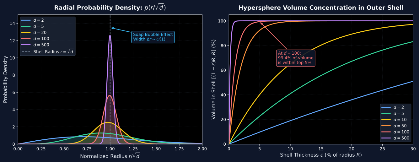
High-dimensional space defies low-dimensional intuition. Two fundamental phenomena dictate the behavior of high-dimensional Gaussian random variables $\mathbf{x} \sim \mathcal{N}(\mathbf{0}, \mathbf{I}_d)$:

Phenomenon 1: Concentration on the Sphere Surface (The "Soap Bubble" Effect)

The squared norm $\|\mathbf{x}\|^2 = \sum_{i=1}^d x_i^2$ is the sum of $d$ independent $\chi_1^2$ random variables.

• $\mathbb{E}[\|\mathbf{x}\|^2] = d$
• $\operatorname{Var}(\|\mathbf{x}\|^2) = 2d$

The relative fluctuation of the radius is:

$$\frac{\sqrt{\operatorname{Var}(\|\mathbf{x}\|)}}{\mathbb{E}[\|\mathbf{x}\|]} \approx \frac{\sqrt{2d} / (2\sqrt{d})}{\sqrt{d}} = \frac{1}{\sqrt{2d}} \xrightarrow{d \to \infty} 0$$

By Bernstein's inequality:

$$\mathbb{P}\left( \left| \frac{\|\mathbf{x}\|^2}{d} - 1 \right| \ge \epsilon \right) \le 2 \exp\left( - \frac{d \epsilon^2}{8} \right)$$

Almost all the probability mass of a $d$-dimensional standard Gaussian vector resides inside a thin hyperspherical shell of radius $\sqrt{d}$ and thickness $\mathcal{O}(1)$.

Phenomenon 2: Quasi-Orthogonality of Random Vectors

Let $\mathbf{u}, \mathbf{v} \sim \mathcal{N}(\mathbf{0}, \mathbf{I}_d)$ be independent random vectors. The cosine of their angle $\theta$ is:

$$\cos \theta = \frac{\mathbf{u}^\top \mathbf{v}}{\|\mathbf{u}\| \|\mathbf{v}\|} \approx \frac{\sum_{i=1}^d u_i v_i}{d}$$

Since $u_i v_i$ are independent random variables with mean 0 and variance 1:

$$\mathbb{E}[\cos \theta] = 0, \quad \operatorname{Var}(\cos \theta) \approx \frac{1}{d}$$ $$\mathbb{P}(|\cos \theta| \ge \epsilon) \le 2 \exp\left( -\frac{d \epsilon^2}{2} \right)$$

In high dimensions, any two independent random vectors are almost certainly orthogonal: $\theta \approx \pi/2 \pm \mathcal{O}(d^{-1/2})$.

---

3. Self-Averaging in Statistical Physics & Deep Learning

3.1 Mathematical Definition of Self-Averaging

In disordered physical systems (e.g., spin glasses, random alloys) or deep neural networks initialized with random weights, the Hamiltonian $\mathcal{H}_N(\boldsymbol{\sigma}; \mathbf{J})$ or empirical loss $\hat{\mathcal{L}}_N(\mathbf{w}; \mathcal{D})$ depends on quenched random variables $\mathbf{J} \sim P(\mathbf{J})$ or initial weights $\mathbf{W} \sim P(\mathbf{W})$.

---

3.2 Quenched vs. Annealed Averages

When averaging thermodynamic quantities over disorder $\mathcal{D} = \{\mathbf{x}_i, y_i\}_{i=1}^n$ or random weights $\mathbf{W}$:

1. Annealed Average (Disorder in Thermal Equilibrium)

The disorder degrees of freedom fluctuate on the same timescale as the system variables:

$$F_{\mathrm{ann}} = -\frac{1}{\beta} \ln \mathbb{E}_{\mathcal{D}}[Z(\mathcal{D})] = -\frac{1}{\beta} \ln \int d\mathcal{D} P(\mathcal{D}) \int d\mathbf{w} \, e^{-\beta \mathcal{H}(\mathbf{w}; \mathcal{D})}$$

2. Quenched Average (Frozen Disorder)

The disorder is fixed permanently, and the system reaches thermal equilibrium for that specific realization:

$$F_{\mathrm{quenched}} = -\frac{1}{\beta} \mathbb{E}_{\mathcal{D}}[\ln Z(\mathcal{D})] = -\frac{1}{\beta} \int d\mathcal{D} P(\mathcal{D}) \ln \left( \int d\mathbf{w} \, e^{-\beta \mathcal{H}(\mathbf{w}; \mathcal{D})} \right)$$

By Jensen's inequality, since the logarithm is strictly concave:

$$\mathbb{E}[\ln Z] \le \ln \mathbb{E}[Z] \implies F_{\mathrm{quenched}} \ge F_{\mathrm{ann}}$$

In deep learning, the dataset $\mathcal{D}$ and the random initialization $\mathbf{W}_0$ act as quenched disorder. Because the training loss is self-averaging in the wide limit, the quenched free energy equals the typical free energy of a single randomly initialized network.

---

4. The Infinite-Width Limit: Neural Network Gaussian Processes (NNGP)

In 1995, Radford Neal proved that single-hidden-layer Bayesian neural networks converge to Gaussian Processes as width $N \to \infty$. In 2018, Lee et al. and Matthews et al. extended this result to deep multi-layer architectures.

4.1 Multi-Layer Perceptron Setup

Consider an $L$-hidden-layer fully connected neural network defined recursively:

$$\begin{aligned} f^{(1)}_i(\mathbf{x}) &= \sum_{j=1}^{d_0} W^{(1)}_{ij} x_j + b^{(1)}_i \\ h^{(l)}_i(\mathbf{x}) &= \sigma\left( f^{(l)}_i(\mathbf{x}) \right), \quad l = 1, \dots, L \\ f^{(l+1)}_i(\mathbf{x}) &= \frac{\sigma_w}{\sqrt{N_l}} \sum_{j=1}^{N_l} W^{(l+1)}_{ij} h^{(l)}_j(\mathbf{x}) + \sigma_b b^{(l+1)}_i \end{aligned}$$

Where:

• $\mathbf{x} \in \mathbb{R}^{d_0}$ is the input vector.
• $N_l$ is the width (number of neurons) of layer $l$.
• $W^{(l)}_{ij} \overset{\mathrm{i.i.d.}}{\sim} \mathcal{N}(0, 1)$ are Gaussian weights scaled by $\frac{\sigma_w}{\sqrt{N_l}}$.
• $b^{(l)}_i \overset{\mathrm{i.i.d.}}{\sim} \mathcal{N}(0, 1)$ are Gaussian biases scaled by $\sigma_b$.
• $\sigma: \mathbb{R} \to \mathbb{R}$ is a non-linear activation function (e.g., ReLU, GeLU, erf).

---

4.2 Step-by-Step Induction for NNGP Convergence

We prove by induction on layer index $l$ that for any finite collection of inputs $\{\mathbf{x}_1, \dots, \mathbf{x}_k\}$, the joint pre-activations $\left( f^{(l)}_i(\mathbf{x}_1), \dots, f^{(l)}_i(\mathbf{x}_k) \right)$ converge in distribution to a zero-mean multivariate Gaussian as $N_1, \dots, N_{l-1} \to \infty$.

Base Case: Layer $l = 1$

For any input $\mathbf{x}$, the pre-activation is:

$$f^{(1)}_i(\mathbf{x}) = \sum_{j=1}^{d_0} W^{(1)}_{ij} x_j + \sigma_b b^{(1)}_i$$

Since $W^{(1)}_{ij}$ and $b^{(1)}_i$ are independent Gaussians, $f^{(1)}_i(\mathbf{x})$ is an exact linear combination of independent zero-mean Gaussians. For any two inputs $\mathbf{x}, \mathbf{x}'$:

$$\mathbb{E}[f^{(1)}_i(\mathbf{x})] = 0$$ $$\begin{aligned} \mathcal{K}^{(1)}(\mathbf{x}, \mathbf{x}') &\equiv \mathbb{E}\left[ f^{(1)}_i(\mathbf{x}) f^{(1)}_i(\mathbf{x}') \right] \\ &= \sum_{j=1}^{d_0} \sum_{k=1}^{d_0} x_j x'_k \, \mathbb{E}[W^{(1)}_{ij} W^{(1)}_{ik}] + \sigma_b^2 \mathbb{E}[b^{(1)}_i b^{(1)}_i] \\ &= \frac{\sigma_w^2}{d_0} \mathbf{x}^\top \mathbf{x}' + \sigma_b^2 \end{aligned}$$

For distinct neurons $i \neq i'$, $\mathbb{E}[f^{(1)}_i(\mathbf{x}) f^{(1)}_{i'}(\mathbf{x}')] = 0$. Thus, $f^{(1)}_i \sim \mathcal{GP}(0, \mathcal{K}^{(1)})$ independently for each $i$.

Inductive Step: Layer $l \to l+1$

Assume that as $N_{l-1} \to \infty$, the pre-activations $\left( f^{(l)}_1, \dots, f^{(l)}_{N_l} \right)$ are i.i.d. draws from a zero-mean Gaussian Process with covariance $\mathcal{K}^{(l)}(\mathbf{x}, \mathbf{x}')$.

Conditioned on the previous layer activations $h^{(l)}_j(\mathbf{x}) = \sigma(f^{(l)}_j(\mathbf{x}))$, the pre-activation of neuron $i$ at layer $l+1$ is:

$$f^{(l+1)}_i(\mathbf{x}) = \frac{\sigma_w}{\sqrt{N_l}} \sum_{j=1}^{N_l} W^{(l+1)}_{ij} h^{(l)}_j(\mathbf{x}) + \sigma_b b^{(l+1)}_i$$

Conditioned on $h^{(l)}$, $f^{(l+1)}_i(\mathbf{x})$ is a sum of $N_l$ independent random terms:

$$\zeta_j(\mathbf{x}) \equiv \frac{\sigma_w}{\sqrt{N_l}} W^{(l+1)}_{ij} h^{(l)}_j(\mathbf{x})$$

The conditional mean is zero: $\mathbb{E}[\zeta_j(\mathbf{x}) \mid h^{(l)}] = 0$. The conditional covariance is:

$$\begin{aligned} \operatorname{Cov}\left( f^{(l+1)}_i(\mathbf{x}), f^{(l+1)}_i(\mathbf{x}') \,\middle|\, h^{(l)} \right) &= \sigma_b^2 + \frac{\sigma_w^2}{N_l} \sum_{j=1}^{N_l} \sum_{k=1}^{N_l} h^{(l)}_j(\mathbf{x}) h^{(l)}_k(\mathbf{x}') \, \mathbb{E}\left[ W^{(l+1)}_{ij} W^{(l+1)}_{ik} \right] \\ &= \sigma_b^2 + \sigma_w^2 \left( \frac{1}{N_l} \sum_{j=1}^{N_l} h^{(l)}_j(\mathbf{x}) h^{(l)}_j(\mathbf{x}') \right) \\ &= \sigma_b^2 + \sigma_w^2 \left( \frac{1}{N_l} \sum_{j=1}^{N_l} \sigma(f^{(l)}_j(\mathbf{x})) \sigma(f^{(l)}_j(\mathbf{x}')) \right) \end{aligned}$$

By the Strong Law of Large Numbers, as the width $N_l \to \infty$, the empirical average over neurons converges almost surely to the statistical expectation:

$$\frac{1}{N_l} \sum_{j=1}^{N_l} \sigma(f^{(l)}_j(\mathbf{x})) \sigma(f^{(l)}_j(\mathbf{x}')) \xrightarrow{\text{a.s.}} \mathbb{E}_{f^{(l)} \sim \mathcal{GP}(0, \mathcal{K}^{(l)})}\left[ \sigma(f^{(l)}(\mathbf{x})) \sigma(f^{(l)}(\mathbf{x}')) \right]$$

By the Multidimensional Central Limit Theorem, $f^{(l+1)}_i(\mathbf{x})$ converges in distribution to an unconditional zero-mean Gaussian process $f^{(l+1)}_i \sim \mathcal{GP}(0, \mathcal{K}^{(l+1)})$ with recursive kernel:

---

4.3 Closed-Form Analytical Kernels: The Arc-Cosine / ReLU Case

For the Rectified Linear Unit (ReLU) activation $\sigma(z) = \max(0, z)$, Cho and Saul (2009) derived the exact closed-form evaluation of $\mathcal{T}_{\mathrm{ReLU}}$.

Let $u, v \sim \mathcal{N}\left( \mathbf{0}, \begin{pmatrix} K_{xx} & K_{xx'} \\ K_{xx'} & K_{x'x'} \end{pmatrix} \right)$. Define the correlation angle:

$$\theta \equiv \arccos\left( \frac{K_{xx'}}{\sqrt{K_{xx} K_{x'x'}}} \right), \quad \theta \in [0, \pi]$$

Using polar transformation $u = \sqrt{K_{xx}} r \cos \phi$, $v = \sqrt{K_{x'x'}} r \cos(\phi - \theta)$:

$$\begin{aligned} \mathcal{T}_{\mathrm{ReLU}}(K_{xx}, K_{x'x'}, K_{xx'}) &= \frac{\sqrt{K_{xx} K_{x'x'}}}{2\pi} \left[ \sin \theta + (\pi - \theta) \cos \theta \right] \\ &= \frac{\sqrt{K_{xx} K_{x'x'}}}{2\pi} \left[ \sqrt{1 - \left(\frac{K_{xx'}}{\sqrt{K_{xx} K_{x'x'}}}\right)^2} + \left( \pi - \arccos\frac{K_{xx'}}{\sqrt{K_{xx} K_{x'x'}}} \right) \frac{K_{xx'}}{\sqrt{K_{xx} K_{x'x'}}} \right] \end{aligned}$$

For the derivative kernel $\dot{\mathcal{K}}^{(l)}(\mathbf{x}, \mathbf{x}') \equiv \sigma_w^2 \mathbb{E}[\sigma'(u) \sigma'(v)]$ (where $\sigma'(z) = \Theta(z)$ is the Heaviside step function):

$$\dot{\mathcal{T}}_{\mathrm{ReLU}}(K_{xx}, K_{x'x'}, K_{xx'}) = \frac{1}{2\pi} (\pi - \theta) = \frac{1}{2\pi} \left( \pi - \arccos\frac{K_{xx'}}{\sqrt{K_{xx} K_{x'x'}}} \right)$$

---

5. Dynamic Thermodynamic Limit: The Neural Tangent Kernel (NTK)

While the NNGP describes Bayesian neural networks at initialization, real neural networks are trained with gradient descent. Jacot, Gabriel, and Hongler (NeurIPS 2018) discovered that in the infinite-width limit, gradient descent dynamics become entirely linear and analytically solvable through the Neural Tangent Kernel (NTK).

$\frac{df(x_{\text{test}})}{dt} = -\Theta(x_{\text{test}}, X_{\text{train}}) \left( f(X_{\text{train}}) - y \right)$

5.1 Derivation of Continuous-Time Gradient Flow

Let $f(\mathbf{x}; \boldsymbol{\theta})$ be the neural network output parameterized by $\boldsymbol{\theta} \in \mathbb{R}^P$. We train on a dataset $\mathcal{D} = \{(\mathbf{x}_i, y_i)\}_{i=1}^n$ with Mean Squared Error (MSE) loss:

$$\mathcal{L}(\boldsymbol{\theta}) = \frac{1}{2} \sum_{i=1}^n \left( f(\mathbf{x}_i; \boldsymbol{\theta}) - y_i \right)^2$$

Under continuous-time gradient descent ($\frac{d\boldsymbol{\theta}_t}{dt} = -\eta \nabla_{\boldsymbol{\theta}} \mathcal{L}(\boldsymbol{\theta}_t)$ with learning rate $\eta$):

$$\frac{d\boldsymbol{\theta}_t}{dt} = -\eta \sum_{i=1}^n \left( f(\mathbf{x}_i; \boldsymbol{\theta}_t) - y_i \right) \nabla_{\boldsymbol{\theta}} f(\mathbf{x}_i; \boldsymbol{\theta}_t)$$

By the multivariate chain rule, the time derivative of the network output at an arbitrary query point $\mathbf{x}$ is:

$$\begin{aligned} \frac{d f(\mathbf{x}; \boldsymbol{\theta}_t)}{dt} &= \left( \nabla_{\boldsymbol{\theta}} f(\mathbf{x}; \boldsymbol{\theta}_t) \right)^\top \frac{d\boldsymbol{\theta}_t}{dt} \\ &= -\eta \sum_{i=1}^n \left[ \nabla_{\boldsymbol{\theta}} f(\mathbf{x}; \boldsymbol{\theta}_t)^\top \nabla_{\boldsymbol{\theta}} f(\mathbf{x}_i; \boldsymbol{\theta}_t) \right] \left( f(\mathbf{x}_i; \boldsymbol{\theta}_t) - y_i \right) \end{aligned}$$

In vector notation across the training set $\mathbf{X} \in \mathbb{R}^{n \times d_0}$ with predictions $\mathbf{f}_t = f(\mathbf{X}; \boldsymbol{\theta}_t) \in \mathbb{R}^n$ and labels $\mathbf{y} \in \mathbb{R}^n$:

$$\frac{d \mathbf{f}_t}{dt} = -\eta \hat{\boldsymbol{\Theta}}_t(\mathbf{X}, \mathbf{X}) (\mathbf{f}_t - \mathbf{y})$$

---

5.2 The Two Pillars of Infinite-Width NTK Theory

As the widths $N_1, \dots, N_L \to \infty$:

1. Self-Averaging at Initialization ($t = 0$)

The empirical kernel converges in probability to a deterministic, invariant kernel $\mathbf{\Theta}_\infty$:

$$\hat{\Theta}_0(\mathbf{x}, \mathbf{x}') \xrightarrow{P} \Theta_\infty(\mathbf{x}, \mathbf{x}') \quad \text{as } N \to \infty$$

2. Kernel Freeze / Lazy Training Regime ($t > 0$)

Throughout gradient descent training, the parameters move by at most $\|\boldsymbol{\theta}_t - \boldsymbol{\theta}_0\| = \mathcal{O}(1/\sqrt{N})$. The relative change in the empirical tangent kernel is strictly bounded:

$$\sup_{t \ge 0} \left\| \hat{\boldsymbol{\Theta}}_t - \hat{\boldsymbol{\Theta}}_0 \right\|_F = \mathcal{O}\left(\frac{1}{\sqrt{N}}\right) \xrightarrow{N \to \infty} 0$$

Because $\hat{\boldsymbol{\Theta}}_t \equiv \mathbf{\Theta}_\infty$ is constant in time, the non-linear gradient flow reduces to a linear ordinary differential equation:

$$\frac{d \mathbf{f}_t}{dt} = -\eta \mathbf{\Theta}_\infty (\mathbf{f}_t - \mathbf{y})$$

Subtracting $\mathbf{y}$ from both sides:

$$\frac{d(\mathbf{f}_t - \mathbf{y})}{dt} = -\eta \mathbf{\Theta}_\infty (\mathbf{f}_t - \mathbf{y}) \implies \mathbf{f}_t - \mathbf{y} = \exp\left( -\eta \mathbf{\Theta}_\infty t \right) (\mathbf{f}_0 - \mathbf{y})$$

$f_t(X_{\text{train}}) = y + e^{-\eta \Theta_{\text{train}} t} (f_0(X_{\text{train}}) - y)$

At convergence ($t \to \infty$), assuming $\mathbf{\Theta}_\infty(\mathbf{X}, \mathbf{X})$ is strictly positive definite:

---

5.3 Step-by-Step Derivation of the Recursive NTK Formula

We derive the exact recursive expression for $\Theta^{(L+1)}(\mathbf{x}, \mathbf{x}')$ across hidden layers.

Recall the parameter set $\boldsymbol{\theta} = \bigcup_{l=1}^{L+1} \{ \mathbf{W}^{(l)}, \mathbf{b}^{(l)} \}$. The empirical NTK decomposes as a sum of layer-wise contributions:

$$\hat{\Theta}^{(L+1)}(\mathbf{x}, \mathbf{x}') = \sum_{l=1}^{L+1} \left[ \left\langle \frac{\partial f(\mathbf{x})}{\partial \mathbf{W}^{(l)}}, \frac{\partial f(\mathbf{x}')}{\partial \mathbf{W}^{(l)}} \right\rangle + \left\langle \frac{\partial f(\mathbf{x})}{\partial \mathbf{b}^{(l)}}, \frac{\partial f(\mathbf{x}')}{\partial \mathbf{b}^{(l)}} \right\rangle \right]$$

Let $f(\mathbf{x}) \equiv f^{(L+1)}(\mathbf{x})$. By backpropagation:

$$\frac{\partial f(\mathbf{x})}{\partial W^{(l+1)}_{ij}} = \frac{\partial f(\mathbf{x})}{\partial f^{(l+1)}_i(\mathbf{x})} \frac{\partial f^{(l+1)}_i(\mathbf{x})}{\partial W^{(l+1)}_{ij}} = \delta^{(l+1)}_i(\mathbf{x}) \frac{\sigma_w}{\sqrt{N_l}} h^{(l)}_j(\mathbf{x})$$

where $\delta^{(l)}_i(\mathbf{x}) \equiv \frac{\partial f(\mathbf{x})}{\partial f^{(l)}_i(\mathbf{x})}$. The backward recursion is:

$$\delta^{(l)}_j(\mathbf{x}) = \sum_{k=1}^{N_{l+1}} \delta^{(l+1)}_k(\mathbf{x}) \frac{\sigma_w}{\sqrt{N_l}} W^{(l+1)}_{kj} \sigma'\left( f^{(l)}_j(\mathbf{x}) \right)$$

Evaluating the inner product for weight matrix $\mathbf{W}^{(l+1)}$:

$$\begin{aligned} \left\langle \frac{\partial f(\mathbf{x})}{\partial \mathbf{W}^{(l+1)}}, \frac{\partial f(\mathbf{x}')}{\partial \mathbf{W}^{(l+1)}} \right\rangle &= \sum_{i=1}^{N_{l+1}} \sum_{j=1}^{N_l} \left( \delta^{(l+1)}_i(\mathbf{x}) \frac{\sigma_w}{\sqrt{N_l}} h^{(l)}_j(\mathbf{x}) \right) \left( \delta^{(l+1)}_i(\mathbf{x}') \frac{\sigma_w}{\sqrt{N_l}} h^{(l)}_j(\mathbf{x}') \right) \\ &= \sigma_w^2 \left( \sum_{i=1}^{N_{l+1}} \delta^{(l+1)}_i(\mathbf{x}) \delta^{(l+1)}_i(\mathbf{x}') \right) \left( \frac{1}{N_l} \sum_{j=1}^{N_l} h^{(l)}_j(\mathbf{x}) h^{(l)}_j(\mathbf{x}') \right) \end{aligned}$$

In the infinite-width limit:

1. The forward term converges to the NNGP kernel: $$\frac{1}{N_l} \sum_{j=1}^{N_l} h^{(l)}_j(\mathbf{x}) h^{(l)}_j(\mathbf{x}') \xrightarrow{\text{a.s.}} \mathcal{K}^{(l)}(\mathbf{x}, \mathbf{x}')$$
2. The backward term satisfies the recursive relation: $$\sum_{j=1}^{N_l} \delta^{(l)}_j(\mathbf{x}) \delta^{(l)}_j(\mathbf{x}') \xrightarrow{\text{a.s.}} \dot{\mathcal{K}}^{(l)}(\mathbf{x}, \mathbf{x}') \left( \sum_{k=1}^{N_{l+1}} \delta^{(l+1)}_k(\mathbf{x}) \delta^{(l+1)}_k(\mathbf{x}') \right)$$

Combining forward and backward recursions produces the NTK Master Recursion Formula:

---

6. Quantitative Non-Asymptotic Rates: Eldan, Mikulincer & Schramm (COLT 2021)

While classical NNGP and NTK theorems assert that neural networks converge to Gaussian processes as $N \to \infty$, physical and engineering implementations operate at finite width $N < \infty$. How fast does this convergence occur in function space?

Ronen Eldan, Dan Mikulincer, and Tselil Schramm (COLT 2021) established the first non-asymptotic, quantitative convergence rates in transportation distance.

6.1 Function Space Transportation Metrics

Let $\mathcal{C}(\mathbb{S}^{d-1})$ be the Banach space of continuous functions on the unit sphere equipped with the supremum norm $\|f\|_\infty = \sup_{\mathbf{x} \in \mathbb{S}^{d-1}} |f(\mathbf{x})|$.

The Wasserstein-1 (Kantorovich-Rubinstein) distance between the law of a finite-width network $\mu_N = \operatorname{Law}(f_N)$ and the Gaussian process measure $\gamma = \mathcal{GP}(0, \mathcal{K})$ is:

$$\mathcal{W}_1(\mu_N, \gamma) \equiv \sup_{\substack{\Psi: \mathcal{C}(\mathbb{S}^{d-1}) \to \mathbb{R} \\ \|\Psi\|_{\mathrm{Lip}} \le 1}} \left| \mathbb{E}_{f \sim \mu_N}[\Psi(f)] - \mathbb{E}_{g \sim \gamma}[\Psi(g)] \right|$$

where $\|\Psi\|_{\mathrm{Lip}} = \sup_{f \neq g} \frac{|\Psi(f) - \Psi(g)|}{\|f - g\|_\infty} \le 1$.

---

6.2 The Eldan-Mikulincer-Schramm Convergence Theorem

6.3 Proof Strategy via Infinite-Dimensional Malliavin-Stein Exchangeable Pairs

The proof constructs an exchangeable pair $(f_N, f_N')$ by resampling a single hidden neuron $i^* \sim \operatorname{Uniform}(\{1, \dots, N\})$ with fresh parameters $(\mathbf{w}'_{i^*}, a'_{i^*})$.

The conditional change in the network function is:

$$\mathbb{E}[f_N' - f_N \mid f_N] = -\frac{1}{N} f_N$$

By constructing an infinite-dimensional Stein operator $\mathcal{A} \Psi(f) = \Delta_{\mathcal{K}} \Psi(f) - \langle f, \nabla \Psi(f) \rangle_{\mathcal{H}}$ on the Reproducing Kernel Hilbert Space (RKHS) $\mathcal{H}$, the error decomposes into second-order operator fluctuations bounded by $\mathcal{O}(N^{-1/2})$ via the classical Berry-Esseen inequality on Hilbert spaces.

This proves that the relative error of approximating a finite-width network by its Gaussian process limit scales precisely as:

$$\text{Approximation Error} \sim \mathcal{O}\left( \frac{1}{\sqrt{N}} \right)$$

matching the thermodynamic fluctuation rate of physical ensembles.

---

7. Asymptotic Variance and Mini-Batch SGD under LLN/CLT

Stochastic Gradient Descent (SGD) introduces a second layer of large-number asymptotics: sampling mini-batches $B_t \subset \{1, \dots, n\}$ from a training dataset of size $n$.

$\nabla L_B(\theta) = \nabla L(\theta) + \xi_t, \quad \mathbb{E}[\xi_t] = 0, \quad \text{Cov}(\xi_t) = \frac{\Sigma(\theta)}{B}$

7.1 The Mini-Batch Central Limit Theorem

At parameter state $\boldsymbol{\theta}$, let $\nabla \ell_i(\boldsymbol{\theta})$ be the gradient on datapoint $i$. The full dataset gradient is $\nabla \mathcal{L}(\boldsymbol{\theta}) = \frac{1}{n} \sum_{i=1}^n \nabla \ell_i(\boldsymbol{\theta})$.

When we draw a mini-batch $B \subset \{1, \dots, n\}$ of size $|B| = b$ uniformly with replacement, the mini-batch gradient is:

$$\mathbf{g}_B(\boldsymbol{\theta}) = \frac{1}{b} \sum_{k \in B} \nabla \ell_k(\boldsymbol{\theta})$$

By the Multidimensional Central Limit Theorem, as batch size $b \to \infty$ with $b \ll n$:

$$\sqrt{b} \left( \mathbf{g}_B(\boldsymbol{\theta}) - \nabla \mathcal{L}(\boldsymbol{\theta}) \right) \xrightarrow{d} \mathcal{N}\left( \mathbf{0}, \mathbf{\Sigma}(\boldsymbol{\theta}) \right)$$

where $\mathbf{\Sigma}(\boldsymbol{\theta}) \in \mathbb{R}^{P \times P}$ is the empirical gradient covariance matrix:

$$\mathbf{\Sigma}(\boldsymbol{\theta}) \equiv \frac{1}{n} \sum_{i=1}^n \left( \nabla \ell_i(\boldsymbol{\theta}) - \nabla \mathcal{L}(\boldsymbol{\theta}) \right) \left( \nabla \ell_i(\boldsymbol{\theta}) - \nabla \mathcal{L}(\boldsymbol{\theta}) \right)^\top$$

---

7.2 Continuous-Time Stochastic Differential Equation (SDE) Limit

For small learning rate $\eta \ll 1$, the discrete update $\boldsymbol{\theta}_{k+1} = \boldsymbol{\theta}_k - \eta \mathbf{g}_{B_k}(\boldsymbol{\theta}_k)$ converges weakly to the continuous Itô Stochastic Differential Equation:

$$d\boldsymbol{\theta}_t = -\nabla \mathcal{L}(\boldsymbol{\theta}_t) \, dt + \sqrt{\frac{\eta}{b}} \mathbf{\Sigma}^{1/2}(\boldsymbol{\theta}_t) \, d\mathbf{W}_t$$

where $\mathbf{W}_t$ is standard $P$-dimensional Brownian motion.

Fluctuation-Dissipation Relation in SGD

Comparing this to the physical Langevin equation $d\mathbf{x}_t = -\nabla U(\mathbf{x}_t) dt + \sqrt{2 k_B T} d\mathbf{W}_t$, we identify the effective SGD temperature:

$$T_{\mathrm{eff}} = \frac{\eta}{2 b}$$

• Increasing learning rate $\eta$ or decreasing batch size $b$ increases thermal noise.
• The ratio $\frac{\eta}{b}$ acts as the thermodynamic temperature controlling exploration across non-convex loss valleys.

---

7.3 Asymptotic Covariance: The Continuous Lyapunov Equation

Near a local minimum $\boldsymbol{\theta}^*$ where $\nabla \mathcal{L}(\boldsymbol{\theta}^*) = \mathbf{0}$, we approximate the loss by its quadratic expansion $\mathcal{L}(\boldsymbol{\theta}) \approx \frac{1}{2} (\boldsymbol{\theta} - \boldsymbol{\theta}^*)^\top \mathbf{H} (\boldsymbol{\theta} - \boldsymbol{\theta}^*)$, with Hessian $\mathbf{H} = \nabla^2 \mathcal{L}(\boldsymbol{\theta}^*)$.

The linearized SDE is an Ornstein-Uhlenbeck process:

$$d(\boldsymbol{\theta}_t - \boldsymbol{\theta}^*) = -\mathbf{H} (\boldsymbol{\theta}_t - \boldsymbol{\theta}^*) \, dt + \sqrt{\frac{\eta}{b}} \mathbf{\Sigma}_*^{1/2} \, d\mathbf{W}_t$$

where $\mathbf{\Sigma}_* = \mathbf{\Sigma}(\boldsymbol{\theta}^*)$. The stationary covariance matrix $\mathbf{C} \equiv \lim_{t \to \infty} \mathbb{E}[(\boldsymbol{\theta}_t - \boldsymbol{\theta}^*)(\boldsymbol{\theta}_t - \boldsymbol{\theta}^*)^\top]$ satisfies the continuous Lyapunov equation:

7.4 Polyak-Ruppert Averaging and Quenched CLT (JMLR 2024–2026)

Recent works in JMLR (Li et al., 2026; Singh et al., 2025) establish quenched Central Limit Theorems for the Polyak-Ruppert tail-averaged estimator $\bar{\boldsymbol{\theta}}_T = \frac{1}{T} \sum_{t=1}^T \boldsymbol{\theta}_t$:

$$\sqrt{T} (\bar{\boldsymbol{\theta}}_T - \boldsymbol{\theta}^*) \xrightarrow{d} \mathcal{N}\left( \mathbf{0}, \mathbf{H}^{-1} \mathbf{\Sigma}_* \mathbf{H}^{-1} \right)$$

Remarkably, the asymptotic variance $\mathbf{H}^{-1} \mathbf{\Sigma}_* \mathbf{H}^{-1}$ is independent of the learning rate $\eta$ and matches the statistical Cramér-Rao efficiency lower bound!

---

8. Beyond Infinite-Width: Field Theory & 1/N Expansions for Bayesian Networks

Despite its mathematical elegance, the infinite-width limit ($N \to \infty$) suffers from a fundamental limitation: representations do not evolve. Because $\sup_t \|\hat{\boldsymbol{\Theta}}_t - \hat{\boldsymbol{\Theta}}_0\| \to 0$, the network behaves as a fixed linear kernel machine and cannot perform feature learning.

To understand feature learning, representation adaptation, and finite-size generalization, we must compute $1/N$ perturbative corrections to the partition function (Pacelli et al., Nature Machine Intelligence 2023; Roberts, Yaida & Hanin, 2022).

---

8.1 The Bayesian Neural Network Partition Function

Consider a Bayesian neural network with dataset $\mathcal{D} = \{(\mathbf{x}_a, y_a)\}_{a=1}^P$. The joint posterior partition function is:

$$\mathcal{Z} = \int d\mathbf{W} \, d\mathbf{b} \, P_0(\mathbf{W}, \mathbf{b}) \exp\left( -\frac{\beta}{2} \sum_{a=1}^P \left( f(\mathbf{x}_a; \mathbf{W}, \mathbf{b}) - y_a \right)^2 \right)$$

where $P_0(\mathbf{W}, \mathbf{b}) = \prod_{l=1}^L \exp\left( -\frac{N_l}{2\sigma_w^2} \operatorname{Tr}(\mathbf{W}^{(l)} {\mathbf{W}^{(l)}}^\top) - \frac{1}{2\sigma_b^2} \|\mathbf{b}^{(l)}\|^2 \right)$ is the Gaussian prior.

---

8.2 The Hubbard-Stratonovich Transformation to Collective Field $Q_{ab}$

Integrating out the microscopic Gaussian weights $\mathbf{W}^{(l)}$ introduces a collective matrix field: the empirical layer-wise Gram matrix $Q_{ab}^{(l)} \equiv \frac{1}{N_l} \sum_{j=1}^{N_l} h^{(l)}_j(\mathbf{x}_a) h^{(l)}_j(\mathbf{x}_b)$.

By inserting the functional identity:

$$1 = \int \mathcal{D}\mathbf{Q}^{(l)} \, \delta\left( N_l \mathbf{Q}^{(l)} - \mathbf{h}^{(l)} {\mathbf{h}^{(l)}}^\top \right) = \int \mathcal{D}\mathbf{Q}^{(l)} \mathcal{D}\tilde{\mathbf{Q}}^{(l)} \exp\left( i \operatorname{Tr}\left[ \tilde{\mathbf{Q}}^{(l)} \left( N_l \mathbf{Q}^{(l)} - \mathbf{h}^{(l)} {\mathbf{h}^{(l)}}^\top \right) \right] \right)$$

the partition function transforms into an effective field theory:

$$\mathcal{Z} = \int \prod_{l=1}^L \mathcal{D}\mathbf{Q}^{(l)} \mathcal{D}\tilde{\mathbf{Q}}^{(l)} \exp\left( - S_{\mathrm{eff}}[\mathbf{Q}, \tilde{\mathbf{Q}}] \right)$$

where the effective action scales with layer width $N$:

$$S_{\mathrm{eff}}[\mathbf{Q}, \tilde{\mathbf{Q}}] = N \left( -i \sum_{l=1}^L \operatorname{Tr}(\tilde{\mathbf{Q}}^{(l)} \mathbf{Q}^{(l)}) + \sum_{l=1}^L \mathcal{W}_l(\tilde{\mathbf{Q}}^{(l)}, \mathbf{Q}^{(l-1)}) \right) + \frac{\beta}{2} \sum_{a=1}^P (f_a - y_a)^2$$

---

8.3 Saddle-Point (Mean Field) and Gaussian Free Field ($N \to \infty$)

As $N \to \infty$, the path integral $\mathcal{Z} = \int \mathcal{D}\mathbf{Q} \, e^{-N S_{\mathrm{eff}}[\mathbf{Q}]}$ is dominated by the saddle-point condition:

$$\frac{\delta S_{\mathrm{eff}}}{\delta \mathbf{Q}^{(l)}} = 0, \quad \frac{\delta S_{\mathrm{eff}}}{\delta \tilde{\mathbf{Q}}^{(l)}} = 0$$

The saddle-point solution $\mathbf{Q}_*^{(l)}$ satisfies the deterministic recursive equation:

$$\mathbf{Q}_*^{(l)} = \mathcal{K}_{\mathrm{NNGP}}^{(l)}$$

At $N = \infty$, fluctuations around $\mathbf{Q}_*$ vanish, recovering the Gaussian Process (free field theory).

---

8.4 Systematic $1/N$ Expansion & Feynman Diagram Vertex Corrections

For large but finite width $N < \infty$, we expand the collective field $\mathbf{Q} = \mathbf{Q}_* + \frac{1}{\sqrt{N}} \delta \mathbf{Q}$:

$$S_{\mathrm{eff}}[\mathbf{Q}] = N S_0[\mathbf{Q}_*] + \frac{1}{2} \delta \mathbf{Q}^\top \mathbf{\Delta}^{-1} \delta \mathbf{Q} + \frac{1}{\sqrt{N}} \frac{V_3}{3!} (\delta \mathbf{Q})^3 + \frac{1}{N} \frac{V_4}{4!} (\delta \mathbf{Q})^4 + \mathcal{O}(N^{-3/2})$$

Where:

• $\mathbf{\Delta}$ is the Gaussian propagator (fluctuation covariance of the kernel).
• $V_3$ is the 3-point interaction vertex (skewness).
• $V_4$ is the 4-point interaction vertex (connected 4-point correlator / kurtosis).

The connected 4-point correlator of neuron pre-activations:

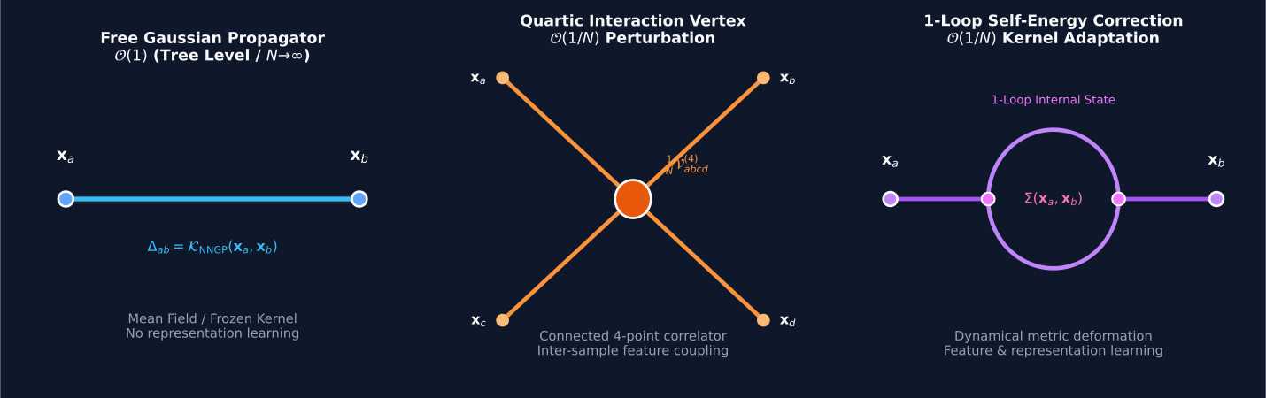
$$\left\langle f_i(\mathbf{x}_a) f_i(\mathbf{x}_b) f_j(\mathbf{x}_c) f_j(\mathbf{x}_d) \right\rangle_c \equiv \left\langle f_i(\mathbf{x}_a) f_i(\mathbf{x}_b) f_j(\mathbf{x}_c) f_j(\mathbf{x}_d) \right\rangle - \mathcal{K}_{ab} \mathcal{K}_{cd} - \mathcal{K}_{ac} \mathcal{K}_{bd} - \mathcal{K}_{ad} \mathcal{K}_{bc}$$

evaluates to:

$$\left\langle f_i(\mathbf{x}_a) f_i(\mathbf{x}_b) f_j(\mathbf{x}_c) f_j(\mathbf{x}_d) \right\rangle_c = \frac{1}{N} \mathcal{V}^{(4)}_{abcd} + \mathcal{O}\left(\frac{1}{N^2}\right)$$

---

9. Classical Statistical Mechanics vs. Deep Learning: Master Correspondence

The following table summarizes the structural equivalence between classical statistical mechanics and infinite-width deep learning:

---

10. Summary & Open Frontiers

Core Takeaways

1. Large Numbers Tame Complexity: In both physical systems ($10^{23}$ particles) and overparameterized neural networks ($N \to \infty$), microscopic randomness concentrates into deterministic macroscopic observables via the Law of Large Numbers and saddle-point integration.
2. The NNGP & NTK Limits: At infinite width, randomly initialized neural networks are mathematically equivalent to Gaussian processes (NNGP), and their training dynamics under gradient descent linearize according to a static kernel (NTK).
3. Finite-Width Fluctuation Theory: Finite networks converge to their infinite-width limits at a rate of $\mathcal{O}(N^{-1/2})$ in Wasserstein-1 distance.
4. SGD as a Thermodynamic Process: Mini-batch SGD behaves as an Ornstein-Uhlenbeck diffusion around minima with effective temperature $T_{\mathrm{eff}} = \eta / (2b)$, leading to stationary covariance governed by the Lyapunov equation.
5. Feature Learning as an Interacting Field Theory: Real deep networks learn features precisely because $N < \infty$. The $1/N$ corrections introduce 4-point Feynman diagram interactions that deform data representations during training.

---

11. Practice Problems with Step-by-Step Solutions

Solution to Problem 1:

Step 1: Multiplicity
Let $N_+$ be the number of dipoles with $\sigma_i = +1$ and $N_-$ be the number with $\sigma_i = -1$.

$$N_+ + N_- = N, \quad N_+ - N_- = M = -\frac{E}{\mu B} \implies N_+ = \frac{N - E/(\mu B)}{2}, \quad N_- = \frac{N + E/(\mu B)}{2}$$

The multiplicity is:

$$\Omega(E) = \binom{N}{N_+} = \frac{N!}{N_+! \, N_-!}$$

Step 2: Entropy with Next-to-Leading Order Stirling Corrections
Using $\ln K! = K \ln K - K + \frac{1}{2}\ln(2\pi K) + \frac{1}{12K} + \mathcal{O}(K^{-2})$:

$$\begin{aligned} \ln \Omega(E) &= \ln N! - \ln N_+! - \ln N_-! \\ &= N \ln N - N_+ \ln N_+ - N_- \ln N_- + \frac{1}{2} \ln\left( \frac{N}{2\pi N_+ N_-} \right) + \frac{1}{12}\left( \frac{1}{N} - \frac{1}{N_+} - \frac{1}{N_-} \right) + \mathcal{O}(N^{-2}) \end{aligned}$$

Let $m = M/N = -E / (N \mu B) \in (-1, 1)$, so $N_\pm = \frac{N(1 \pm m)}{2}$:

$$S(E) = N k_B \left[ \ln 2 - \frac{1+m}{2}\ln(1+m) - \frac{1-m}{2}\ln(1-m) \right] - \frac{k_B}{2}\ln\left( \frac{\pi N (1-m^2)}{2} \right) - \frac{k_B}{3N(1-m^2)} + \mathcal{O}(N^{-2})$$

Step 3: Temperature and Finite-Size Correction
Using $\frac{\partial m}{\partial E} = -\frac{1}{N \mu B}$:

$$\begin{aligned} \frac{1}{T} &= \frac{\partial S}{\partial E} = \frac{\partial m}{\partial E} \frac{\partial S}{\partial m} \\ &= -\frac{1}{N \mu B} \left( -N k_B \frac{1}{2} \ln\left( \frac{1+m}{1-m} \right) + \frac{k_B m}{1-m^2} - \frac{2 k_B m}{3N(1-m^2)^2} + \mathcal{O}(N^{-2}) \right) \\ &= \frac{k_B}{2\mu B} \ln\left( \frac{1+m}{1-m} \right) - \frac{k_B m}{N \mu B (1-m^2)} + \mathcal{O}(N^{-2}) \end{aligned}$$

The first term is the standard thermodynamic relation $m = -\tanh\left(\frac{\mu B}{k_B T}\right)$. The second term shows that for finite $N$, fluctuations reduce the effective magnitude of the magnetization by an order $\mathcal{O}(1/N)$.

---

Solution to Problem 2:

Step 1: Residual Dynamics
The differential equation for the single training point prediction is:

$$\frac{d f(\mathbf{x}_1; \boldsymbol{\theta}_t)}{dt} = -\eta \Theta_\infty(\mathbf{x}_1, \mathbf{x}_1) \left( f(\mathbf{x}_1; \boldsymbol{\theta}_t) - y_1 \right)$$

Let $\epsilon(t) = f(\mathbf{x}_1; \boldsymbol{\theta}_t) - y_1$. Then $\frac{d\epsilon(t)}{dt} = -\eta \Theta_\infty(\mathbf{x}_1, \mathbf{x}_1) \epsilon(t)$, yielding:

$$\epsilon(t) = \epsilon(0) \exp\left( -\eta \Theta_\infty(\mathbf{x}_1, \mathbf{x}_1) t \right) = (f(\mathbf{x}_1; \boldsymbol{\theta}_0) - y_1) e^{-\eta \Theta_\infty(\mathbf{x}_1, \mathbf{x}_1) t}$$

The training error decays exponentially with characteristic convergence time:

$$\tau = \frac{1}{\eta \Theta_\infty(\mathbf{x}_1, \mathbf{x}_1)}$$

Step 2: Test Point Trajectory
For test input $\mathbf{x}^*$:

$$\frac{d f(\mathbf{x}^*; \boldsymbol{\theta}_t)}{dt} = -\eta \Theta_\infty(\mathbf{x}^*, \mathbf{x}_1) \left( f(\mathbf{x}_1; \boldsymbol{\theta}_t) - y_1 \right) = -\eta \Theta_\infty(\mathbf{x}^*, \mathbf{x}_1) (f(\mathbf{x}_1; \boldsymbol{\theta}_0) - y_1) e^{-\eta \Theta_\infty(\mathbf{x}_1, \mathbf{x}_1) t}$$

Integrating from $0$ to $t$:

$$\begin{aligned} f(\mathbf{x}^*; \boldsymbol{\theta}_t) &= f(\mathbf{x}^*; \boldsymbol{\theta}_0) - \eta \Theta_\infty(\mathbf{x}^*, \mathbf{x}_1) (f(\mathbf{x}_1; \boldsymbol{\theta}_0) - y_1) \int_0^t e^{-\eta \Theta_\infty(\mathbf{x}_1, \mathbf{x}_1) s} \, ds \\ &= f(\mathbf{x}^*; \boldsymbol{\theta}_0) + \frac{\Theta_\infty(\mathbf{x}^*, \mathbf{x}_1)}{\Theta_\infty(\mathbf{x}_1, \mathbf{x}_1)} \left( 1 - e^{-\eta \Theta_\infty(\mathbf{x}_1, \mathbf{x}_1) t} \right) \left( y_1 - f(\mathbf{x}_1; \boldsymbol{\theta}_0) \right) \end{aligned}$$

Step 3: Asymptotic Generalization
As $t \to \infty$, taking expectation over initialization ($f_0 \sim \mathcal{GP}(0, \mathcal{K})$ with zero mean):

$$\mathbb{E}[f_\infty(\mathbf{x}^*)] = \frac{\Theta_\infty(\mathbf{x}^*, \mathbf{x}_1)}{\Theta_\infty(\mathbf{x}_1, \mathbf{x}_1)} y_1$$

If the true underlying target function is $y(\mathbf{x}^*)$, the generalization error on $\mathbf{x}^*$ is:

$$\text{Error}(\mathbf{x}^*) = \left| \frac{\Theta_\infty(\mathbf{x}^*, \mathbf{x}_1)}{\Theta_\infty(\mathbf{x}_1, \mathbf{x}_1)} y_1 - y(\mathbf{x}^*) \right|$$

Generalization succeeds if and only if the normalized kernel similarity $\frac{\Theta_\infty(\mathbf{x}^*, \mathbf{x}_1)}{\Theta_\infty(\mathbf{x}_1, \mathbf{x}_1)}$ accurately mirrors the true functional correlation $\frac{y(\mathbf{x}^*)}{y_1}$.

---

12. References & Key Literature