7. Phase Space Evolution, Liouville's Theorem & Continuous Flow Matching

"The phase space is a strange and beautiful world where every point represents an entire universe in a specific microscopic state, and time evolution is nothing other than an incompressible fluid flow." — Ludwig Boltzmann & J. Willard Gibbs

In the previous chapters, we analyzed static equilibrium ensembles, free energy landscapes, and the stochastic dynamics of Brownian particles via the Langevin equation and the Fluctuation-Dissipation theorem. In this chapter, we take a foundational step: we investigate the exact deterministic laws governing how probability distributions evolve through continuous dynamical systems.

We begin in the classical realm of 19th-century statistical mechanics with Hamiltonian mechanics, the phase space probability density $\rho(q, p, t)$, and Liouville's Theorem, which establishes the profound incompressibility of Hamiltonian phase space flows. We then bridge this classical physics to 21st-century deep learning. By relaxing the Hamiltonian constraint to general vector fields on Euclidean and Riemannian manifolds, we arrive at the General Probability Continuity Equation, the engine behind Continuous Normalizing Flows (CNFs), and Flow Matching (Lipman et al., 2023).

Finally, we establish the exact mathematical dictionary linking Stochastic Differential Equations (SDEs), Fokker-Planck Equations, Deterministic Probability Flow ODEs, and Optimal Transport Flow Matching.

---

1. Hamiltonian Mechanics and Phase Space Geometry

1.1 The Canonical Coordinates and Symplectic Structure

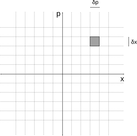
Consider a classical physical system with $d$ degrees of freedom. In Newtonian mechanics, the state is specified by positions $q \in \mathbb{R}^d$ and velocities $\dot{q} \in \mathbb{R}^d$. In Hamiltonian mechanics, the state is elevated to a point in a $2d$-dimensional phase space $\Gamma \cong \mathbb{R}^{2d}$, parameterized by canonical generalized coordinates $q = (q_1, \dots, q_d)^\top$ and their conjugate momenta $p = (p_1, \dots, p_d)^\top$.

The state vector is denoted by:

$$z = \begin{pmatrix} q \\ p \end{pmatrix} \in \Gamma \cong \mathbb{R}^{2d}$$

The total energy of the system is governed by the scalar Hamiltonian function $H(q, p, t): \mathbb{R}^{2d} \times \mathbb{R} \to \mathbb{R}$. For standard mechanical systems with kinetic energy $T(p)$ and potential energy $V(q)$:

$$H(q, p) = \sum_{i=1}^d \frac{p_i^2}{2m_i} + V(q_1, \dots, q_d)$$

The time evolution of the microstate $z(t)$ is governed by Hamilton's Canonical Equations of Motion:

$$\begin{aligned} \dot{q}_i &= \frac{\partial H}{\partial p_i} \\ \dot{p}_i &= -\frac{\partial H}{\partial q_i} \qquad \text{for } i \in \{1, \dots, d\} \end{aligned}$$

We can express these equations compactly using the canonical symplectic matrix $J \in \mathbb{R}^{2d \times 2d}$:

$$\dot{z} = J \nabla_z H(z)$$

where:

$$J = \begin{pmatrix} 0 & I_d \\ -I_d & 0 \end{pmatrix}, \quad J^\top = -J = J^{-1}, \quad J^2 = -I_{2d}$$

---

1.2 Phase Space Probability Density $\rho(q, p, t)$

In statistical mechanics, we almost never know the exact microscopic state $z(0)$ of a system containing $N \sim 10^{23}$ particles. Instead, following Josiah Willard Gibbs, we define a statistical ensemble: a collection of an infinite number of virtual, non-interacting copies of the system, each evolving according to Hamilton's equations under identical macroscopic constraints.

We define the phase space probability density $\rho(q, p, t) = \rho(z, t)$ such that the probability $dP$ of finding the system in an infinitesimal phase volume element $d^{2d}z = dq \, dp = \prod_{i=1}^d dq_i \, dp_i$ at time $t$ is:

$$dP = \rho(q, p, t) \, dq_1 \dots dq_d \, dp_1 \dots dp_d = \rho(z, t) \, d^{2d}z$$

The density is non-negative and normalized over the entire phase space $\Gamma$:

$$\rho(z, t) \ge 0, \quad \int_{\Gamma} \rho(z, t) \, d^{2d}z = 1 \quad \forall t \ge 0$$

---

2. Liouville's Theorem: Incompressibility of Phase Space

2.1 The Divergence-Free Nature of Hamiltonian Vector Fields

Consider the phase space velocity vector field $v(z) \in \mathbb{R}^{2d}$:

$$v(z) = \dot{z} = \begin{pmatrix} \dot{q} \\ \dot{p} \end{pmatrix} = \begin{pmatrix} \nabla_p H \\ -\nabla_q H \end{pmatrix}$$

Let us compute the phase space divergence of this velocity field $\nabla_z \cdot v(z)$:

$$\begin{aligned} \nabla_z \cdot v(z) &= \sum_{i=1}^d \frac{\partial \dot{q}_i}{\partial q_i} + \sum_{i=1}^d \frac{\partial \dot{p}_i}{\partial p_i} \\ &= \sum_{i=1}^d \frac{\partial}{\partial q_i} \left( \frac{\partial H}{\partial p_i} \right) + \sum_{i=1}^d \frac{\partial}{\partial p_i} \left( -\frac{\partial H}{\partial q_i} \right) \\ &= \sum_{i=1}^d \left( \frac{\partial^2 H}{\partial q_i \partial p_i} - \frac{\partial^2 H}{\partial p_i \partial q_i} \right) \end{aligned}$$

By Clairaut-Schwarz Theorem on the equality of mixed partial derivatives (assuming $H \in C^2$):

$$\frac{\partial^2 H}{\partial q_i \partial p_i} = \frac{\partial^2 H}{\partial p_i \partial q_i} \implies \nabla_z \cdot v(z) \equiv 0$$

---

2.2 Geometric Conservation of Phase Space Volume

Let $\Phi_t: \Gamma \to \Gamma$ be the Hamiltonian flow map that maps an initial condition $z_0$ to its state at time $t$:

$$z(t) = \Phi_t(z_0)$$

Consider an arbitrary domain $\Omega_0 \subset \Gamma$ of initial conditions, which evolves under the flow into $\Omega_t = \Phi_t(\Omega_0)$. The volume of this domain at time $t$ is:

$$\operatorname{Vol}(\Omega_t) = \int_{\Omega_t} d^{2d}z = \int_{\Omega_0} |\det M(t)| \, d^{2d}z_0$$

where $M(t) = \frac{\partial z(t)}{\partial z_0} = \frac{\partial \Phi_t(z_0)}{\partial z_0} \in \mathbb{R}^{2d \times 2d}$ is the Jacobian matrix of the flow map.

To see how the Jacobian determinant evolves, we invoke Jacobi's Formula for matrix derivatives:

$$\frac{d}{dt} \det(M(t)) = \det(M(t)) \operatorname{Tr}\left( \dot{M}(t) M(t)^{-1} \right)$$

Differentiating the equation of motion $\dot{z}(t) = v(z(t))$ with respect to $z_0$:

$$\dot{M}(t) = \frac{d}{dt} \left( \frac{\partial z(t)}{\partial z_0} \right) = \frac{\partial v(z(t))}{\partial z(t)} \frac{\partial z(t)}{\partial z_0} = \left[ \nabla_z v(z(t)) \right] M(t)$$

Multiplying by $M(t)^{-1}$ on the right:

$$\dot{M}(t) M(t)^{-1} = \nabla_z v(z(t))$$

Taking the trace of both sides:

$$\operatorname{Tr}\left( \dot{M}(t) M(t)^{-1} \right) = \operatorname{Tr}\left( \nabla_z v(z(t)) \right) = \nabla_z \cdot v(z(t))$$

Substituting this back into Jacobi's Formula:

$$\frac{d}{dt} \det(M(t)) = \det(M(t)) \left( \nabla_z \cdot v(z(t)) \right)$$

Since $\nabla_z \cdot v = 0$ for all Hamiltonian systems:

$$\frac{d}{dt} \det(M(t)) = 0 \implies \det(M(t)) = \det(M(0)) = \det(I_{2d}) = 1$$

Therefore, the phase space volume is strictly invariant under Hamiltonian time evolution:

$$\operatorname{Vol}(\Omega_t) = \int_{\Omega_0} 1 \cdot d^{2d}z_0 = \operatorname{Vol}(\Omega_0)$$

---

2.3 The Liouville Equation & Poisson Brackets

Because no systems are created or destroyed, the total probability inside a co-moving volume $\Omega_t$ is strictly conserved:

$$\frac{d}{dt} \int_{\Omega_t} \rho(z, t) \, d^{2d}z = 0$$

Transforming the integral back to the fixed initial domain $\Omega_0$:

$$\frac{d}{dt} \int_{\Omega_0} \rho(\Phi_t(z_0), t) \underbrace{\det(M(t))}_{= 1} \, d^{2d}z_0 = \int_{\Omega_0} \frac{d}{dt} \rho(z(t), t) \, d^{2d}z_0 = 0$$

Because this must hold for any arbitrary volume $\Omega_0$, the integrand must vanish identically:

$$\frac{d}{dt} \rho(z(t), t) = 0 \quad \text{(Total / Material Derivative)}$$

Expanding the total time derivative using the multivariate chain rule:

$$\frac{d\rho}{dt} = \frac{\partial \rho}{\partial t} + \sum_{i=1}^d \left( \frac{\partial \rho}{\partial q_i} \dot{q}_i + \frac{\partial \rho}{\partial p_i} \dot{p}_i \right) = \frac{\partial \rho}{\partial t} + \nabla_z \rho \cdot \dot{z} = 0$$

Substituting Hamilton's equations $\dot{q}_i = \frac{\partial H}{\partial p_i}$ and $\dot{p}_i = -\frac{\partial H}{\partial q_i}$:

$$\frac{\partial \rho}{\partial t} + \sum_{i=1}^d \left( \frac{\partial \rho}{\partial q_i} \frac{\partial H}{\partial p_i} - \frac{\partial \rho}{\partial p_i} \frac{\partial H}{\partial q_i} \right) = 0$$

We introduce the Poisson Bracket $\{\cdot, \cdot\}$ between two phase space observables $A(q, p)$ and $B(q, p)$:

$$\{ A, B \} \equiv \sum_{i=1}^d \left( \frac{\partial A}{\partial q_i} \frac{\partial B}{\partial p_i} - \frac{\partial A}{\partial p_i} \frac{\partial B}{\partial q_i} \right)$$

This yields the celebrated Classical Liouville Equation:

$$\frac{\partial \rho}{\partial t} = -\{ \rho, H \}$$

Alternatively, defining the Liouvillian Operator $\hat{L} \equiv -\{ \cdot, H \}$:

$$\frac{\partial \rho}{\partial t} = \hat{L} \rho \implies \rho(t) = e^{\hat{L} t} \rho(0)$$

[!NOTE] Physical Interpretation of Liouville's Theorem

1. Lagrangian Viewpoint (Co-moving observer): As an observer rides along a trajectory $z(t)$ in phase space, the local probability density surrounding them never changes: $\frac{d\rho(z(t), t)}{dt} = 0$.
2. Eulerian Viewpoint (Stationary observer): At a fixed coordinate $z \in \Gamma$, the local density changes at a rate exactly balanced by the advective probability flux: $\frac{\partial \rho}{\partial t} = -\nabla_z \rho \cdot v(z) = -\{ \rho, H \}$.
3. Equilibrium Ensembles: A distribution is stationary ($\frac{\partial \rho}{\partial t} = 0$) if and only if $\{\rho, H\} = 0$. This is automatically satisfied whenever $\rho(q, p) = f(H(q, p))$ depends on coordinates only through the conserved energy $H$, yielding the Microcanonical Ensemble $\rho \propto \delta(H - E)$ and Canonical Ensemble $\rho \propto e^{-\beta H}$.

---

3. The General Probability Continuity Equation

In modern machine learning, statistics, and non-conservative physics, dynamics are not restricted to Hamiltonian vector fields. The vector field $u_t(x) \in \mathbb{R}^d$ can have non-zero divergence ($\nabla \cdot u_t \neq 0$), representing stretching, compression, and arbitrary smooth deformations of space.

3.1 Derivation from Mass Conservation

Let $p_t(x): \mathbb{R}^d \to \mathbb{R}_{\ge 0}$ be a time-dependent probability density over state space $x \in \mathbb{R}^d$, transported by a velocity vector field $u_t(x): \mathbb{R}^d \to \mathbb{R}^d$.

Consider an arbitrary, fixed control volume $V \subset \mathbb{R}^d$ with smooth boundary $\partial V$ and outward unit normal vector $n(x)$.

The total probability mass inside $V$ at time $t$ is:

$$P(V, t) = \int_V p_t(x) \, dx$$

The rate of change of probability inside $V$ must equal the negative net probability flux exiting through the boundary $\partial V$:

$$\frac{d}{dt} \int_V p_t(x) \, dx = - \oint_{\partial V} p_t(x) u_t(x) \cdot n(x) \, dA$$

Applying the Divergence Theorem (Gauss-Ostrogradsky Theorem) to the boundary integral:

$$\oint_{\partial V} p_t(x) u_t(x) \cdot n(x) \, dA = \int_V \nabla \cdot \left( p_t(x) u_t(x) \right) \, dx$$

Since the control volume $V$ is stationary in time:

$$\int_V \left[ \frac{\partial p_t(x)}{\partial t} + \nabla \cdot \left( p_t(x) u_t(x) \right) \right] dx = 0$$

Because this equality holds for every arbitrary volume $V \subset \mathbb{R}^d$, the integrand must vanish everywhere:

$$\frac{\partial p_t(x)}{\partial t} + \nabla \cdot \left( p_t(x) u_t(x) \right) = 0$$

This is the General Eulerian Probability Continuity Equation (or advection equation for conserved probability mass).

---

3.2 Eulerian vs. Lagrangian Decomposition

We can expand the divergence term using the vector product rule $\nabla \cdot (p u) = p (\nabla \cdot u) + u \cdot \nabla p$:

$$\frac{\partial p_t(x)}{\partial t} + u_t(x) \cdot \nabla p_t(x) + p_t(x) \left( \nabla \cdot u_t(x) \right) = 0$$

Recognizing the material derivative along a flow trajectory $\dot{x}(t) = u_t(x(t))$:

$$\frac{d}{dt} p_t(x(t)) = \frac{\partial p_t}{\partial t} + \nabla p_t \cdot \dot{x}(t) = \frac{\partial p_t}{\partial t} + u_t(x) \cdot \nabla p_t(x)$$

Substituting this into the expanded continuity equation yields:

$$\frac{d}{dt} p_t(x(t)) = - p_t(x(t)) \left( \nabla \cdot u_t(x(t)) \right)$$

Dividing both sides by $p_t(x(t)) > 0$ and noting that $\frac{d}{dt} \log p = \frac{1}{p} \frac{dp}{dt}$:

$$\frac{d}{dt} \log p_t(x(t)) = - \nabla \cdot u_t(x(t))$$

[!IMPORTANT] Comparison: Liouville vs. General Continuity Equation

Property	Classical Hamiltonian System (Liouville)	General Machine Learning Flow (CNF / Flow Matching)
State Space	Phase Space $\Gamma = \mathbb{R}^{2d}$ with $(q, p)$	Arbitrary Feature / Latent Space $x \in \mathbb{R}^d$
Velocity Field	$v(z) = J \nabla H(z)$ (Symplectic gradient)	$u_t(x) = v_\theta(x, t)$ (Arbitrary Neural Network)
Divergence	$\nabla \cdot v(z) \equiv 0$ (Incompressible)	$\nabla \cdot u_t(x) \neq 0$ (Compressible / Expansible)
Jacobian Determinant	$\det(M(t)) = 1$	$\det(M(t)) = \exp\left( \int_0^t \nabla \cdot u_s \, ds \right)$
Lagrangian Density	$\frac{d\rho}{dt} = 0$ (Constant along path)	$\frac{d \log p_t}{dt} = -\nabla \cdot u_t(x(t))$ (Changes dynamically)
Continuity PDE	$\frac{\partial \rho}{\partial t} + \nabla \rho \cdot v = 0$	$\frac{\partial p_t}{\partial t} + \nabla \cdot (p_t u_t) = 0$

---

4. Continuous Normalizing Flows (CNFs)

4.1 Pushforward Measures and Continuous Change of Variables

In generative modeling, our objective is to transform an easily sampleable base noise distribution $p_0(x_0) = \mathcal{N}(x_0; 0, I_d)$ into a complex, multi-modal target data distribution $q(x_1) \approx p_{\mathrm{data}}(x_1)$.

Let $\psi_t: \mathbb{R}^d \to \mathbb{R}^d$ be the continuous flow map generated by an Ordinary Differential Equation (ODE) parameterized by a neural network $v_\theta(x, t)$:

$$\frac{d x(t)}{dt} = v_\theta(x(t), t), \quad x(0) = x_0 \sim p_0(x_0)$$

The state at time $t$ is given by integrating the vector field:

$$x(t) = \psi_t(x_0) = x_0 + \int_0^t v_\theta(x(s), s) \, ds$$

The pushforward distribution $p_t = [\psi_t]_\sharp p_0$ satisfies the discrete change-of-variables formula:

$$p_t(x(t)) = p_0(x_0) \left| \det \left( \frac{\partial \psi_t(x_0)}{\partial x_0} \right) \right|^{-1}$$

Taking the logarithm:

$$\log p_t(x(t)) = \log p_0(x_0) - \log \left| \det \left( \frac{\partial \psi_t(x_0)}{\partial x_0} \right) \right|$$

Using our Lagrangian continuity result $\frac{d}{dt} \log p_t(x(t)) = -\nabla \cdot v_\theta(x(t), t)$, we integrate directly from $t=0$ to $t=1$:

$$\log p_1(x(1)) = \log p_0(x(0)) - \int_0^1 \nabla \cdot v_\theta(x(t), t) \, dt$$

---

4.2 Hutchinson's Trace Estimator for Scalable Divergence

The exact divergence $\nabla \cdot v_\theta(x, t) = \operatorname{Tr}\left( \frac{\partial v_\theta}{\partial x} \right)$ requires computing all $d$ diagonal elements of the Jacobian matrix $\frac{\partial v_\theta}{\partial x} \in \mathbb{R}^{d \times d}$. For high-dimensional data (e.g., images with $d = 3 \times 512 \times 512 \approx 7.8 \times 10^5$), computing the full Jacobian requires $d$ backward passes of automatic differentiation, which is computationally prohibitive ($\mathcal{O}(d)$ backward passes).

To solve this, Continuous Normalizing Flows (Chen et al., 2018; Grathwohl et al., 2019 - FFJORD) utilize Hutchinson's Stochastic Trace Estimator.

Let $\epsilon \in \mathbb{R}^d$ be a random noise vector drawn from a zero-mean distribution with covariance identity $\operatorname{Cov}(\epsilon) = \mathbb{E}[\epsilon \epsilon^\top] = I_d$ (such as standard Gaussian $\mathcal{N}(0, I_d)$ or Rademacher distribution $\epsilon_i \in \{-1, +1\}$ with equal probability).

For any square matrix $A \in \mathbb{R}^{d \times d}$:

$$\begin{aligned} \mathbb{E}_{\epsilon} \left[ \epsilon^\top A \epsilon \right] &= \mathbb{E}_{\epsilon} \left[ \operatorname{Tr}\left( \epsilon^\top A \epsilon \right) \right] = \mathbb{E}_{\epsilon} \left[ \operatorname{Tr}\left( A \epsilon \epsilon^\top \right) \right] \\ &= \operatorname{Tr}\left( A \mathbb{E}_{\epsilon} \left[ \epsilon \epsilon^\top \right] \right) = \operatorname{Tr}(A I_d) = \operatorname{Tr}(A) \end{aligned}$$

Setting $A = \frac{\partial v_\theta}{\partial x}$:

$$\nabla \cdot v_\theta(x, t) = \operatorname{Tr}\left( \frac{\partial v_\theta}{\partial x} \right) = \mathbb{E}_{\epsilon \sim \mathcal{N}(0, I_d)} \left[ \epsilon^\top \left( \frac{\partial v_\theta(x, t)}{\partial x} \right) \epsilon \right]$$

---

5. Flow Matching: The Modern Paradigm (Lipman et al., 2023)

Despite the mathematical elegance of CNFs, training them via Maximum Likelihood requires numerically integrating the ODE $x(t)$ and its divergence across the entire time interval $t \in [0, 1]$ for every gradient step. This makes CNF training notoriously slow, unstable, and prone to error accumulation.

Flow Matching (Lipman et al., ICLR 2023; Albergo & Vanden-Eijnden, 2023; Liu et al., 2023) revolutionizes continuous generative modeling by providing a simulation-free objective. It enables training continuous normalizing flows with simple regression losses—completely bypassing numerical ODE integration during training.

---

5.1 The Target Probability Path and Intractable Flow Matching

Let $q(x_1)$ be the empirical data distribution, and $p_0(x_0) = \mathcal{N}(x_0; 0, I)$ be the prior noise distribution.

We desire a time-dependent probability path $p_t(x)$ for $t \in [0, 1]$ such that:

• At $t = 0$: $p_0(x)$ is the known noise distribution.
• At $t = 1$: $p_1(x) \approx q(x_1)$ is the target data distribution.

If we knew the true marginal vector field $u_t(x)$ that generates $p_t(x)$ via the continuity equation:

$$\frac{\partial p_t(x)}{\partial t} + \nabla \cdot \left( p_t(x) u_t(x) \right) = 0$$

We could train a neural network $v_\theta(x, t)$ via the ideal Flow Matching (FM) objective:

$$\mathcal{L}_{\mathrm{FM}}(\theta) = \mathbb{E}_{t \sim \mathcal{U}[0, 1], x \sim p_t(x)} \left[ \| v_\theta(x, t) - u_t(x) \|_2^2 \right]$$

---

5.2 Conditional Flow Matching (CFM)

Lipman et al. (2023) solved this impasse by introducing Conditional Flow Matching (CFM).

Instead of working with the intractable marginal path $p_t(x)$, we condition on individual data points $x_1 \sim q(x_1)$ (or pairs $(x_0, x_1)$). We define simple, tractable conditional probability paths $p_t(x | x_1)$ and corresponding conditional vector fields $u_t(x | x_1)$ that satisfy the conditional continuity equation:

$$\frac{\partial p_t(x | x_1)}{\partial t} + \nabla \cdot \left( p_t(x | x_1) u_t(x | x_1) \right) = 0$$

The marginal quantities are related to the conditional quantities by marginalization:

$$p_t(x) = \int p_t(x | x_1) q(x_1) \, dx_1$$ $$u_t(x) = \int u_t(x | x_1) \frac{p_t(x | x_1) q(x_1)}{p_t(x)} \, dx_1$$

We now define the Conditional Flow Matching (CFM) objective:

$$\mathcal{L}_{\mathrm{CFM}}(\theta) = \mathbb{E}_{t \sim \mathcal{U}[0, 1], x_1 \sim q(x_1), x \sim p_t(x | x_1)} \left[ \| v_\theta(x, t) - u_t(x | x_1) \|_2^2 \right]$$

This objective is completely tractable and simulation-free: we sample $x_1 \sim q(x_1)$, sample $t \sim \mathcal{U}[0, 1]$, sample $x \sim p_t(x | x_1)$, evaluate the closed-form conditional vector field $u_t(x | x_1)$, and compute a standard MSE loss!

---

5.3 Step-by-Step Proof of the CFM Theorem

We now present the complete, rigorous mathematical proof that optimizing the tractable $\mathcal{L}_{\mathrm{CFM}}(\theta)$ is mathematically identical to optimizing the intractable $\mathcal{L}_{\mathrm{FM}}(\theta)$.

Proof:

Expand the squared Euclidean norm in the marginal Flow Matching loss $\mathcal{L}_{\mathrm{FM}}(\theta)$:

$$\begin{aligned} \mathcal{L}_{\mathrm{FM}}(\theta) &= \mathbb{E}_{t, x \sim p_t(x)} \left[ \| v_\theta(x, t) - u_t(x) \|_2^2 \right] \\ &= \int_0^1 dt \int_{\mathbb{R}^d} dx \, p_t(x) \left( \| v_\theta(x, t) \|_2^2 - 2 \langle v_\theta(x, t), u_t(x) \rangle + \| u_t(x) \|_2^2 \right) \end{aligned}$$

Since $\| u_t(x) \|_2^2$ does not depend on the network parameters $\theta$, taking the gradient with respect to $\theta$ yields:

$$\nabla_\theta \mathcal{L}_{\mathrm{FM}}(\theta) = \int_0^1 dt \int_{\mathbb{R}^d} dx \, p_t(x) \left( \nabla_\theta \| v_\theta(x, t) \|_2^2 - 2 \nabla_\theta \langle v_\theta(x, t), u_t(x) \rangle \right)$$

Now examine the cross-term $\int_{\mathbb{R}^d} p_t(x) \langle v_\theta(x, t), u_t(x) \rangle \, dx$. Substitute the definition of the marginal vector field $u_t(x) = \int u_t(x | x_1) \frac{p_t(x | x_1) q(x_1)}{p_t(x)} \, dx_1$:

$$\begin{aligned} \int_{\mathbb{R}^d} p_t(x) \langle v_\theta(x, t), u_t(x) \rangle \, dx &= \int_{\mathbb{R}^d} p_t(x) \left\langle v_\theta(x, t), \int_{\mathbb{R}^d} u_t(x | x_1) \frac{p_t(x | x_1) q(x_1)}{p_t(x)} \, dx_1 \right\rangle dx \\ &= \int_{\mathbb{R}^d} \int_{\mathbb{R}^d} q(x_1) p_t(x | x_1) \langle v_\theta(x, t), u_t(x | x_1) \rangle \, dx \, dx_1 \\ &= \mathbb{E}_{x_1 \sim q(x_1), x \sim p_t(x | x_1)} \left[ \langle v_\theta(x, t), u_t(x | x_1) \rangle \right] \end{aligned}$$

Similarly, for the first term:

$$\begin{aligned} \int_{\mathbb{R}^d} p_t(x) \| v_\theta(x, t) \|_2^2 \, dx &= \int_{\mathbb{R}^d} \left( \int_{\mathbb{R}^d} p_t(x | x_1) q(x_1) \, dx_1 \right) \| v_\theta(x, t) \|_2^2 \, dx \\ &= \int_{\mathbb{R}^d} \int_{\mathbb{R}^d} q(x_1) p_t(x | x_1) \| v_\theta(x, t) \|_2^2 \, dx \, dx_1 \\ &= \mathbb{E}_{x_1 \sim q(x_1), x \sim p_t(x | x_1)} \left[ \| v_\theta(x, t) \|_2^2 \right] \end{aligned}$$

Now, write out the expansion of the Conditional Flow Matching loss $\mathcal{L}_{\mathrm{CFM}}(\theta)$:

$$\begin{aligned} \mathcal{L}_{\mathrm{CFM}}(\theta) &= \mathbb{E}_{t, x_1 \sim q(x_1), x \sim p_t(x | x_1)} \left[ \| v_\theta(x, t) - u_t(x | x_1) \|_2^2 \right] \\ &= \mathbb{E}_{t, x_1, x} \left[ \| v_\theta(x, t) \|_2^2 \right] - 2 \mathbb{E}_{t, x_1, x} \left[ \langle v_\theta(x, t), u_t(x | x_1) \rangle \right] + \mathbb{E}_{t, x_1, x} \left[ \| u_t(x | x_1) \|_2^2 \right] \end{aligned}$$

Taking the gradient with respect to $\theta$:

$$\nabla_\theta \mathcal{L}_{\mathrm{CFM}}(\theta) = \nabla_\theta \mathbb{E}_{t, x_1, x} \left[ \| v_\theta(x, t) \|_2^2 \right] - 2 \nabla_\theta \mathbb{E}_{t, x_1, x} \left[ \langle v_\theta(x, t), u_t(x | x_1) \rangle \right]$$

Matching terms with the gradient of $\mathcal{L}_{\mathrm{FM}}(\theta)$:

$$\nabla_\theta \mathcal{L}_{\mathrm{FM}}(\theta) \equiv \nabla_\theta \mathcal{L}_{\mathrm{CFM}}(\theta)$$

Furthermore, subtracting the two loss functions:

$$\mathcal{L}_{\mathrm{CFM}}(\theta) - \mathcal{L}_{\mathrm{FM}}(\theta) = \mathbb{E}_{t, x_1 \sim q(x_1), x \sim p_t(x | x_1)} \left[ \| u_t(x | x_1) \|_2^2 \right] - \mathbb{E}_{t, x \sim p_t(x)} \left[ \| u_t(x) \|_2^2 \right] \ge 0$$

This difference is a non-negative constant independent of $\theta$. $\blacksquare$

---

5.4 Optimal Transport Paths and Straight-Line Trajectories

What is the optimal choice for the conditional probability path $p_t(x | x_1)$?

Consider the Gaussian conditional path conditioned on both a noise sample $x_0 \sim p_0(x_0) = \mathcal{N}(0, I)$ and a data sample $x_1 \sim q(x_1)$:

$$\psi_t(x_0, x_1) = (1 - t) x_0 + t x_1$$

The conditional vector field along this path is simply the time-derivative:

$$u_t(x | x_0, x_1) = \frac{d}{dt} \psi_t(x_0, x_1) = x_1 - x_0$$

In standard Conditional Flow Matching (Independent Coupling), $x_0 \sim \mathcal{N}(0, I)$ and $x_1 \sim q(x_1)$ are sampled independently: $q(x_0, x_1) = p_0(x_0) q(x_1)$.

In Optimal Transport Conditional Flow Matching (OT-CFM), we sample $(x_0, x_1)$ from the 2-Wasserstein optimal transport plan $\pi(x_0, x_1) \in \Pi(p_0, q)$:

$$\pi^* = \arg\min_{\pi \in \Pi(p_0, q)} \int_{\mathbb{R}^d \times \mathbb{R}^d} \| x_0 - x_1 \|_2^2 \, d\pi(x_0, x_1)$$

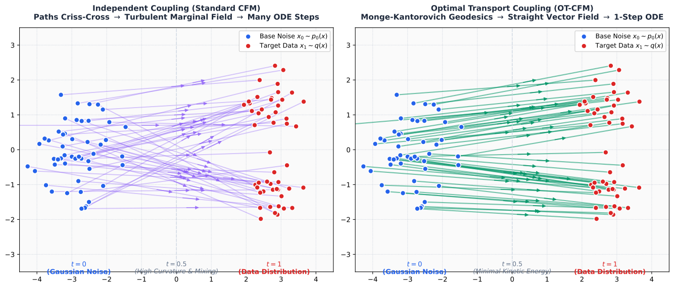
In practice, this is computed over mini-batches using the Hungarian algorithm or Earth Mover's Distance solver.

[!TIP] Why Straight Paths Matter When the trajectories $x(t)$ are straight lines ($u_t(x) = \text{const}$), the velocity field does not change direction along the flow. This allows numerical ODE solvers (e.g., Euler or Heun) to take massive step sizes, generating high-fidelity images in as few as 1 to 4 evaluation steps, compared to 50–1000 steps required by traditional curved diffusion models!

---

6. SDEs vs. ODEs: Stochastic Diffusion vs. Probability Flow ODEs

We now unify stochastic physics (Brownian motion, Langevin dynamics) with deterministic probability flows.

6.1 The Fokker-Planck Equation for Itô SDEs

Consider a general forward Stochastic Differential Equation (SDE) in $\mathbb{R}^d$:

$$dx_t = f(x_t, t) \, dt + g(t) \, dw_t$$

where $f(x, t) \in \mathbb{R}^d$ is the drift coefficient, $g(t) \in \mathbb{R}$ is the scalar diffusion coefficient, and $w_t$ is standard $d$-dimensional Brownian motion ($dw_t \sim \mathcal{N}(0, dt \, I_d)$).

The time evolution of the marginal probability density $p_t(x)$ is governed by the Fokker-Planck Equation (Forward Kolmogorov Equation):

$$\frac{\partial p_t(x)}{\partial t} = - \nabla \cdot \left( f(x, t) p_t(x) \right) + \frac{1}{2} g(t)^2 \nabla^2 p_t(x)$$

where $\nabla^2 p_t(x) = \sum_{i=1}^d \frac{\partial^2 p_t}{\partial x_i^2} = \nabla \cdot (\nabla p_t(x))$ is the spatial Laplacian.

---

6.2 Exact Derivation of the Deterministic Probability Flow ODE

Let us rewrite the second-order diffusion term $\nabla^2 p_t(x)$ in terms of the Stein Score Function $s(x, t) \equiv \nabla_x \log p_t(x)$:

$$\nabla p_t(x) = p_t(x) \nabla_x \log p_t(x)$$

Taking the divergence of both sides:

$$\nabla^2 p_t(x) = \nabla \cdot \left( \nabla p_t(x) \right) = \nabla \cdot \left( p_t(x) \nabla_x \log p_t(x) \right)$$

Substitute this identity back into the Fokker-Planck Equation:

$$\begin{aligned} \frac{\partial p_t(x)}{\partial t} &= - \nabla \cdot \left( f(x, t) p_t(x) \right) + \frac{1}{2} g(t)^2 \nabla \cdot \left( p_t(x) \nabla_x \log p_t(x) \right) \\ &= - \nabla \cdot \left[ p_t(x) \left( f(x, t) - \frac{1}{2} g(t)^2 \nabla_x \log p_t(x) \right) \right] \end{aligned}$$

Rearranging into the standard Continuity Equation form:

$$\frac{\partial p_t(x)}{\partial t} + \nabla \cdot \left( p_t(x) v_t(x) \right) = 0$$

where the deterministic velocity field $v_t(x)$ is defined as:

$$v_t(x) \equiv f(x, t) - \frac{1}{2} g(t)^2 \nabla_x \log p_t(x)$$

This equivalence reveals that Score-based Diffusion Models and Continuous Normalizing Flows are two sides of the same coin:

1. Diffusion models learn the spatial gradient of the log-density $\nabla_x \log p_t(x)$ (the score).
2. Flow Matching models directly learn the velocity field $v_t(x)$ that integrates the continuity equation.

---

7. The Grand Synthesis: Physics vs. Deep Learning Dictionary

The following table summarizes the exact mathematical and conceptual correspondences between Classical Hamiltonian Statistical Mechanics, Stochastic Non-Equilibrium Thermodynamics, and Modern Continuous Generative Modeling.

---

8. Practical Implementation: Flow Matching in PyTorch

Below is a complete, minimal, and fully runnable implementation of Optimal Transport Conditional Flow Matching (OT-CFM) in PyTorch, including Hutchinson trace estimation for log-likelihood evaluation.

import torch
import torch.nn as nn
import torch.optim as optim

class TimeMLP(nn.Module):
    """Time-dependent Vector Field v_theta(x, t)"""
    def __init__(self, dim=2, hidden_dim=128):
        super().__init__()
        self.net = nn.Sequential(
            nn.Linear(dim + 1, hidden_dim),
            nn.SiLU(),
            nn.Linear(hidden_dim, hidden_dim),
            nn.SiLU(),
            nn.Linear(hidden_dim, hidden_dim),
            nn.SiLU(),
            nn.Linear(hidden_dim, dim)
        )
        
    def forward(self, x, t):
        # x: [B, dim], t: [B, 1]
        t_input = t if t.dim() == 2 else t.unsqueeze(-1)
        tx = torch.cat([x, t_input], dim=-1)
        return self.net(tx)

class ConditionalFlowMatcher:
    """Optimal Transport / Linear Conditional Flow Matcher"""
    def __init__(self, sigma_min=1e-4):
        self.sigma_min = sigma_min

    def compute_loss(self, model, x_1):
        """
        x_1: Target data batch [B, dim]
        """
        B, dim = x_1.shape
        x_0 = torch.randn_like(x_1) # Base distribution p_0 ~ N(0, I)
        t = torch.rand(B, 1, device=x_1.device) # t ~ Uniform[0, 1]
        
        # Affine interpolation path: psi_t(x_0, x_1) = (1 - (1 - sigma_min)*t) * x_0 + t * x_1
        # Target vector field: u_t(x|x_0, x_1) = x_1 - (1 - sigma_min) * x_0
        psi_t = (1.0 - (1.0 - self.sigma_min) * t) * x_0 + t * x_1
        u_t = x_1 - (1.0 - self.sigma_min) * x_0
        
        # Neural network prediction
        v_pred = model(psi_t, t)
        
        # CFM Regression Loss
        loss = torch.mean((v_pred - u_t) ** 2)
        return loss

    @torch.no_grad()
    def sample_ode(self, model, num_samples, dim, steps=50, device='cpu'):
        """Euler ODE Integrator: dx = v_theta(x, t) dt from t=0 to 1"""
        x = torch.randn(num_samples, dim, device=device)
        dt = 1.0 / steps
        
        for step in range(steps):
            t_val = step * dt
            t_tensor = torch.full((num_samples, 1), t_val, device=device)
            v = model(x, t_tensor)
            x = x + v * dt # Euler step
            
        return x

def hutchinson_divergence(model, x, t, num_probes=1):
    """
    Computes unbiased estimate of div(v_theta) = Tr(dv/dx) using Hutchinson's estimator
    """
    x.requires_grad_(True)
    v = model(x, t)
    div = torch.zeros(x.shape[0], device=x.device)
    
    for _ in range(num_probes):
        # Rademacher noise eps in {-1, +1}
        eps = torch.randint(0, 2, x.shape, device=x.device).float() * 2.0 - 1.0
        # Vector-Jacobian Product (VJP)
        vjp = torch.autograd.grad(v, x, grad_outputs=eps, create_graph=True)[0]
        div += torch.sum(vjp * eps, dim=-1)
        
    return div / num_probes

---

9. Modern Frontiers (2024–2026)

The principles of Liouville's theorem and continuous flow matching form the bedrock of the most recent breakthroughs in foundation generative models:

---

10. Exercises and Derivations

Exercise 1: Incompressibility of 1D Harmonic Oscillator Flow

Problem: A one-dimensional harmonic oscillator has Hamiltonian $H(q, p) = \frac{p^2}{2m} + \frac{1}{2} k q^2$.

1. Write Hamilton's equations for this system.
2. Solve the equations analytically for $q(t)$ and $p(t)$ given initial conditions $(q_0, p_0)$.
3. Compute the Jacobian matrix $M(t) = \frac{\partial (q(t), p(t))}{\partial (q_0, p_0)}$ and show directly that $\det(M(t)) = 1$ for all $t$.

Solution:

1. Hamilton's equations are: $$\dot{q} = \frac{\partial H}{\partial p} = \frac{p}{m}, \quad \dot{p} = -\frac{\partial H}{\partial q} = -k q$$
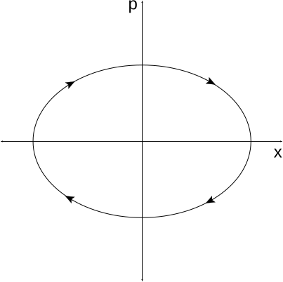
2. Let $\omega = \sqrt{\frac{k}{m}}$. Differentiating $\dot{q}$: $\ddot{q} = \frac{\dot{p}}{m} = -\frac{k}{m} q = -\omega^2 q$. The general solutions are: $$\begin{aligned} q(t) &= q_0 \cos(\omega t) + \frac{p_0}{m \omega} \sin(\omega t) \\ p(t) &= p_0 \cos(\omega t) - m \omega q_0 \sin(\omega t) \end{aligned}$$
3. The Jacobian matrix is: $$M(t) = \begin{pmatrix} \frac{\partial q(t)}{\partial q_0} & \frac{\partial q(t)}{\partial p_0} \\ \frac{\partial p(t)}{\partial q_0} & \frac{\partial p(t)}{\partial p_0} \end{pmatrix} = \begin{pmatrix} \cos(\omega t) & \frac{1}{m \omega} \sin(\omega t) \\ -m \omega \sin(\omega t) & \cos(\omega t) \end{pmatrix}$$ Computing the determinant: $$\det(M(t)) = (\cos(\omega t))(\cos(\omega t)) - \left( \frac{1}{m \omega} \sin(\omega t) \right) (-m \omega \sin(\omega t)) = \cos^2(\omega t) + \sin^2(\omega t) \equiv 1$$ This proves exact volume preservation $\det(M(t)) = 1$. $\blacksquare$

---

Exercise 2: CFM Loss Gradient for General Exponential Paths

Problem: Consider a general Gaussian conditional probability path:

$$p_t(x | x_1) = \mathcal{N}(x; \mu_t(x_1), \sigma_t^2 I_d)$$

with conditional flow $\psi_t(x_0, x_1) = \mu_t(x_1) + \sigma_t x_0$ where $x_0 \sim \mathcal{N}(0, I_d)$.

1. Derive the conditional vector field $u_t(x | x_1)$ as a function of $x$ and $x_1$.
2. Prove that this vector field satisfies the conditional continuity equation $\frac{\partial p_t}{\partial t} + \nabla \cdot (p_t u_t) = 0$.

Solution:

1. Differentiating $\psi_t(x_0, x_1)$ with respect to $t$: $$\frac{d}{dt} \psi_t(x_0, x_1) = \dot{\mu}_t(x_1) + \dot{\sigma}_t x_0$$ Inverting the flow map for $x_0$: $x_0 = \frac{x - \mu_t(x_1)}{\sigma_t}$. Substituting this into the velocity expression gives: $$u_t(x | x_1) = \dot{\mu}_t(x_1) + \frac{\dot{\sigma}_t}{\sigma_t} \left( x - \mu_t(x_1) \right)$$
2. Let $p_t(x | x_1) = (2\pi \sigma_t^2)^{-d/2} \exp\left( -\frac{\| x - \mu_t(x_1) \|_2^2}{2\sigma_t^2} \right)$. Compute the time derivative of $\log p_t$: $$\frac{\partial \log p_t}{\partial t} = -\frac{d \dot{\sigma}_t}{\sigma_t} + \frac{\dot{\sigma}_t}{\sigma_t^3} \| x - \mu_t \|^2 + \frac{1}{\sigma_t^2} (x - \mu_t)^\top \dot{\mu}_t$$ Compute the spatial gradient: $$\nabla \log p_t = -\frac{x - \mu_t}{\sigma_t^2}$$ Compute the divergence of $u_t$: $$\nabla \cdot u_t = \sum_{i=1}^d \frac{\partial}{\partial x_i} \left( \dot{\mu}_{t,i} + \frac{\dot{\sigma}_t}{\sigma_t} (x_i - \mu_{t,i}) \right) = d \frac{\dot{\sigma}_t}{\sigma_t}$$ Now evaluate the left side of the continuity equation in logarithmic form: $$\begin{aligned} \frac{\partial \log p_t}{\partial t} + u_t \cdot \nabla \log p_t + \nabla \cdot u_t &= \left[ -d \frac{\dot{\sigma}_t}{\sigma_t} + \frac{\dot{\sigma}_t}{\sigma_t^3} \|x-\mu_t\|^2 + \frac{\dot{\mu}_t \cdot (x-\mu_t)}{\sigma_t^2} \right] \\ &\quad + \left( \dot{\mu}_t + \frac{\dot{\sigma}_t}{\sigma_t}(x-\mu_t) \right) \cdot \left( -\frac{x-\mu_t}{\sigma_t^2} \right) + d \frac{\dot{\sigma}_t}{\sigma_t} \\ &= -d \frac{\dot{\sigma}_t}{\sigma_t} + \frac{\dot{\sigma}_t}{\sigma_t^3} \|x-\mu_t\|^2 + \frac{\dot{\mu}_t \cdot (x-\mu_t)}{\sigma_t^2} \\ &\quad - \frac{\dot{\mu}_t \cdot (x-\mu_t)}{\sigma_t^2} - \frac{\dot{\sigma}_t}{\sigma_t^3} \|x-\mu_t\|^2 + d \frac{\dot{\sigma}_t}{\sigma_t} \\ &= 0 \end{aligned}$$ Multiplying by $p_t(x | x_1)$ yields $\frac{\partial p_t}{\partial t} + \nabla \cdot (p_t u_t) = 0$. $\blacksquare$