5. Phase Transitions, Order Parameters & Grokking in Deep Learning

In the study of complex physical systems, macroscopic phenomena—such as the sudden freezing of water into crystalline ice or the spontaneous emergence of bulk magnetization in a cooling iron bar—cannot be understood by examining individual particles in isolation. These phenomena are phase transitions: abrupt, non-analytic transformations in the macroscopic behavior of a system driven by smooth variations in underlying control parameters (such as temperature, pressure, or magnetic field).

Deep learning models operate under a precisely analogous regime. As we scale dataset size $P$, parameter count $N$, sequence length $L$, network depth $D$, or training duration $t$, neural networks do not simply improve smoothly. Instead, they exhibit sharp, qualitative transitions:

• Spontaneous Symmetry Breaking & Specialization: Neurons or attention heads transition from an isotropic, degenerate state into highly specialized functional modes.
• The Interpolation Threshold ($\alpha = P/N \to \alpha_c$): A geometric jamming transition where the training loss landscape reorganizes, accompanied by the double descent of generalization error.
• Grokking (Delayed Generalization): A discontinuous, first-order dynamical phase transition wherein a network abruptly shifts from a high-entropy, memorizing state to a low-complexity, perfectly generalizing state after millions of gradient steps.
• Signal Propagation Collapse: Critical freezing transitions in deep transformers, where representation geometry abruptly collapses into either rank-degenerate subspace alignment or single-token attention freeze-out.

This chapter develops the analytical machinery of statistical mechanics—including Landau's phenomenological theory, the Bogoliubov variational mean-field bound, high-dimensional replica theory, and Derrida's Random Energy Model (REM)—to provide a rigorous, microscopic foundation for these deep learning phenomena.

---

1. Classical Statistical Mechanics vs. Modern Deep Learning

To build a rigorous bridge between statistical physics and deep learning theory, we establish the direct dictionary mapping thermodynamic variables to machine learning observables:

---

2. Theory of Phase Transitions & Landau Theory

2.1 Thermodynamic Limit and the Origin of Non-Analyticity

For any system with a finite number of degrees of freedom $N < \infty$, the partition function $\mathcal{Z}_N(\beta)$ is a finite sum (or well-behaved finite-dimensional integral) of strictly positive, analytic functions:

$$\mathcal{Z}_N(\beta) = \sum_{\sigma \in \Sigma} e^{-\beta \mathcal{H}(\sigma)}$$

Because $\mathcal{Z}_N(\beta) > 0$ for all real $\beta \in (0, \infty)$, the finite-$N$ free energy density:

$$f_N(\beta) = -\frac{1}{\beta N} \ln \mathcal{Z}_N(\beta)$$

is infinitely differentiable ($C^\infty$) with respect to $\beta$ and any external field $h$. Consequently, true phase transitions cannot occur in finite systems.

In machine learning, the thermodynamic limit corresponds to scaling the input dimension $N \to \infty$, dataset size $P \to \infty$, or network width/depth $W, L \to \infty$ while holding critical ratios (such as the sample complexity $\alpha = P/N$ or aspect ratio $\rho = L/D$) constant.

---

2.2 Ehrenfest Classification of Phase Transitions

Phase transitions are classified according to the lowest-order derivative of the free energy density $f(T, h)$ that exhibits a mathematical discontinuity or divergence:

1. First-Order Phase Transitions: The first derivative of the free energy is discontinuous across the transition boundary:

   $$\Delta m = \lim_{h \to 0^+} \left(-\frac{\partial f}{\partial h}\right) - \lim_{h \to 0^-} \left(-\frac{\partial f}{\partial h}\right) \neq 0$$
   • Thermodynamic features: Latent heat, coexistence of distinct metastable phases, hysteresis loops, and a non-zero free energy barrier $\Delta F^\ddagger > 0$ separating competing minima.
   • Deep Learning counterpart: Grokking (where the parameter state tunnels across a free energy barrier from a memorization basin to a generalization basin) and Attention Entropy Collapse in deep transformers.

2. Second-Order (Continuous) Phase Transitions: The first derivative of $f(T, h)$ is continuous, but the second derivative exhibits a discontinuity or divergence:

   $$\chi = -\frac{\partial^2 f}{\partial h^2} = \beta N \left( \langle m^2 \rangle - \langle m \rangle^2 \right) \xrightarrow[T \to T_c]{} \infty$$
   • Thermodynamic features: Divergence of the spatial correlation length $\xi \propto |T - T_c|^{-\nu}$, critical slowing down, scale invariance, and universal critical exponents.
   • Deep Learning counterpart: Spontaneous symmetry breaking in weight initialization, bifurcation of student-teacher networks, and the jamming transition at the interpolation capacity $\alpha = P/N = 1$.

---

2.3 Order Parameters and Spontaneous Symmetry Breaking

Let a physical or computational system possess a microscopic Hamiltonian $\mathcal{H}(W)$ invariant under a global symmetry group $G$ (e.g., the $\mathbb{Z}_2$ spin-flip symmetry $W \to -W$, or the permutation group $S_K$ of hidden units):

$$\mathcal{H}(g \cdot W) = \mathcal{H}(W), \quad \forall g \in G$$

An order parameter $\phi \in \mathbb{R}^k$ is a macroscopic observable defined such that:

1. $\phi = 0$ in the symmetric, disordered, high-temperature phase.
2. $\phi \neq 0$ in the broken-symmetry, ordered, low-temperature phase.

When $T < T_c$, although the Gibbs measure $\mathcal{P}(W) = \frac{1}{\mathcal{Z}} e^{-\beta \mathcal{H}(W)}$ remains formally symmetric under $G$, the system in the thermodynamic limit spontaneously settles into a single pure thermodynamic state $\langle W \rangle_\alpha$, breaking the symmetry. The free energy barrier between disjoint symmetric ground states scales as:

$$\Delta F \sim \mathcal{O}(N) \xrightarrow[N \to \infty]{} \infty$$

rendering transitions between pure states impossible on any finite physical timescale (ergodicity breaking).

---

2.4 Mathematical Formulation of Landau Theory

Landau's phenomenological theory posits that in the vicinity of a critical point $T_c$, the macroscopic free energy density $f(\phi; T, h)$ can be systematically expanded as an analytic power series in the scalar order parameter $\phi$, constrained strictly by the underlying symmetries of the system.

Assuming an inversion symmetry $\phi \to -\phi$ in the absence of an external conjugate field $h$:

$$f(\phi; T, h) = f_0(T) + \frac{a(T)}{2} \phi^2 + \frac{b(T)}{4} \phi^4 + \frac{c(T)}{6} \phi^6 - h \phi + \mathcal{O}(\phi^8)$$

where $f_0(T)$ is the background free energy of the disordered phase. Near the critical temperature $T_c$, we expand the quadratic coefficient to leading order:

$$a(T) = a_0 (T - T_c), \quad a_0 > 0$$

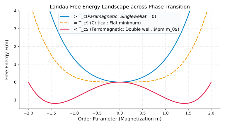
Analytical Derivation: Continuous vs. Discontinuous Landau Minima

The equilibrium value of $\phi$ satisfies the Euler-Lagrange saddle-point condition $\frac{\partial f}{\partial \phi} = 0$:

$$\frac{\partial f}{\partial \phi} = a_0(T - T_c)\phi + b \phi^3 + c \phi^5 - h = 0$$

Case 1: Continuous Phase Transition ($b > 0$, $c \ge 0$, $h = 0$)

For $T > T_c$, $a(T) > 0$; the only real root is $\phi^* = 0$, representing a stable disordered minimum with $\frac{\partial^2 f}{\partial \phi^2}\Big|_{\phi=0} = a_0(T - T_c) > 0$.

For $T < T_c$, $a(T) < 0$; $\phi = 0$ becomes an unstable local maximum. Solving for the non-trivial roots:

$$a_0(T - T_c)\phi + b \phi^3 = 0 \implies \phi^*(T) = \pm \sqrt{\frac{a_0(T_c - T)}{b}} \propto (T_c - T)^\beta$$

This yields the classical mean-field critical exponent:

$$\beta = \frac{1}{2}$$

The magnetic susceptibility $\chi = \frac{\partial \phi}{\partial h}\Big|_{h=0}$ diverges upon approaching $T_c$:

$$\chi(T) = \left[ \frac{\partial^2 f}{\partial \phi^2} \right]^{-1} = \begin{cases} \dfrac{1}{a_0(T - T_c)}, & T > T_c \quad (\gamma = 1) \\[1.2em] \dfrac{1}{2a_0(T_c - T)}, & T < T_c \quad (\gamma' = 1) \end{cases}$$

Case 2: First-Order Phase Transition ($b < 0$, $c > 0$, $h = 0$)

When $b = -|b| < 0$, the quartic term destabilizes the potential, requiring stabilization by the positive sextic term $c > 0$:

$$f(\phi) = f_0 + \frac{a_0(T - T_c)}{2}\phi^2 - \frac{|b|}{4}\phi^4 + \frac{c}{6}\phi^6$$

Setting $\frac{\partial f}{\partial \phi} = \phi \left( a(T) - |b|\phi^2 + c\phi^4 \right) = 0$, the secondary local minima are located at:

$$\phi^2 = \frac{|b| + \sqrt{b^2 - 4 a(T) c}}{2c}$$

A first-order transition occurs at the coexistence temperature $T_{\mathrm{coex}} > T_c$ where the free energy of the ordered state precisely equals that of the disordered state ($f(\phi^*) = f(0) = f_0$). Solving $f(\phi^*) = f_0$ and $\frac{\partial f}{\partial \phi}\Big|_{\phi^*} = 0$ simultaneously yields:

$$\begin{aligned} T_{\mathrm{coex}} &= T_c + \frac{3 b^2}{16 a_0 c} \\ \phi^*(T_{\mathrm{coex}}) &= \pm \sqrt{\frac{3 |b|}{4 c}} \neq 0 \end{aligned}$$

---

3. Mean Field Theory & Self-Consistent Effective Fields

Mean Field Theory (MFT) approximates complex, many-body interacting systems by replacing the fluctuating microscopic interactions experienced by each degree of freedom with an average, self-consistent effective field.

3.1 The Variational Principle (Bogoliubov-Feynman Inequality)

Let $\mathcal{H}(W)$ be the intractable true Hamiltonian of our learning system, with true partition function $\mathcal{Z} = \int dW \, e^{-\beta \mathcal{H}(W)}$ and true free energy $F = -\beta^{-1} \ln \mathcal{Z}$.

Let $\mathcal{H}_0(W; \theta)$ be a family of tractable reference Hamiltonians parameterized by variational parameters $\theta$. The trial partition function and trial free energy are $\mathcal{Z}_0 = \int dW \, e^{-\beta \mathcal{H}_0(W)}$ and $F_0 = -\beta^{-1} \ln \mathcal{Z}_0$.

Proof:

Using the definition of the true partition function:

$$\begin{aligned} \mathcal{Z} &= \int dW \, e^{-\beta \mathcal{H}(W)} = \int dW \, e^{-\beta \mathcal{H}_0(W)} e^{-\beta (\mathcal{H}(W) - \mathcal{H}_0(W))} \\ &= \mathcal{Z}_0 \int dW \, \frac{e^{-\beta \mathcal{H}_0(W)}}{\mathcal{Z}_0} e^{-\beta (\mathcal{H}(W) - \mathcal{H}_0(W))} = \mathcal{Z}_0 \left\langle e^{-\beta (\mathcal{H} - \mathcal{H}_0)} \right\rangle_0 \end{aligned}$$

Taking the natural logarithm and applying Jensen's inequality ($\ln \langle e^X \rangle \ge \langle X \rangle$ due to the strict concavity of the logarithm):

$$\ln \mathcal{Z} = \ln \mathcal{Z}_0 + \ln \left\langle e^{-\beta (\mathcal{H} - \mathcal{H}_0)} \right\rangle_0 \ge \ln \mathcal{Z}_0 - \beta \langle \mathcal{H} - \mathcal{H}_0 \rangle_0$$

Multiplying by $-\beta^{-1}$ reverses the inequality, completing the proof:

$$F = -\frac{1}{\beta} \ln \mathcal{Z} \le -\frac{1}{\beta} \ln \mathcal{Z}_0 + \langle \mathcal{H} - \mathcal{H}_0 \rangle_0 = F_{\mathrm{var}}$$

In modern machine learning, this is the exact foundation of Variational Autoencoders (VAEs) and Variational Bayesian Inference, where $F_{\mathrm{var}}$ is the negative Evidence Lower Bound ($-\mathrm{ELBO}$).

---

3.2 Microscopic Derivation of the Curie-Weiss Mean Field Equation

Consider the fully connected (infinite-range) Ising ferromagnet of $N$ binary spins $\sigma_i \in \{-1, +1\}$:

$$\mathcal{H}(\sigma) = -\frac{J}{2N} \sum_{i=1}^N \sum_{j=1}^N \sigma_i \sigma_j - h \sum_{i=1}^N \sigma_i = -\frac{J N}{2} m(\sigma)^2 - N h m(\sigma)$$

where $m(\sigma) = \frac{1}{N} \sum_{i=1}^N \sigma_i$ is the empirical magnetization.

Exact Solution via Hubbard-Stratonovich Transformation

The partition function is:

$$\mathcal{Z}_N = \sum_{\sigma \in \{-1, 1\}^N} \exp\left( \frac{\beta J N}{2} m(\sigma)^2 + \beta N h m(\sigma) \right)$$

Using the Gaussian Hubbard-Stratonovich identity $\exp(\frac{a}{2} x^2) = \sqrt{\frac{a}{2\pi}} \int_{-\infty}^\infty dy \, \exp(-\frac{a}{2} y^2 + a x y)$ with $a = \beta J N$ and $x = m(\sigma)$:

$$\exp\left( \frac{\beta J N}{2} m(\sigma)^2 \right) = \sqrt{\frac{\beta J N}{2\pi}} \int_{-\infty}^\infty dm' \, \exp\left( -\frac{\beta J N}{2} {m'}^2 + \beta J N m' m(\sigma) \right)$$

Substituting this into $\mathcal{Z}_N$ allows decoupling the sum over spins:

$$\begin{aligned} \mathcal{Z}_N &= \sqrt{\frac{\beta J N}{2\pi}} \int_{-\infty}^\infty dm' \, e^{-\frac{\beta J N}{2} {m'}^2} \sum_{\sigma \in \{-1, 1\}^N} \exp\left( \beta (J m' + h) \sum_{i=1}^N \sigma_i \right) \\ &= \sqrt{\frac{\beta J N}{2\pi}} \int_{-\infty}^\infty dm' \, e^{-\frac{\beta J N}{2} {m'}^2} \prod_{i=1}^N \left( \sum_{\sigma_i = \pm 1} e^{\beta (J m' + h) \sigma_i} \right) \\ &= \sqrt{\frac{\beta J N}{2\pi}} \int_{-\infty}^\infty dm' \, \exp\left( -N \beta \left[ \frac{J}{2} {m'}^2 - \frac{1}{\beta} \ln \left( 2 \cosh(\beta (J m' + h)) \right) \right] \right) \end{aligned}$$

We define the effective free energy functional per spin $g(m'; T, h)$:

$$g(m'; T, h) \equiv \frac{J}{2} {m'}^2 - \frac{1}{\beta} \ln \left( 2 \cosh(\beta (J m' + h)) \right)$$

In the thermodynamic limit $N \to \infty$, Laplace's method (saddle-point approximation) yields the exact free energy density:

$$f(\beta, h) = \lim_{N \to \infty} -\frac{1}{\beta N} \ln \mathcal{Z}_N = \min_{m'} g(m'; T, h)$$

The saddle-point condition $\frac{\partial g}{\partial m'} = 0$ produces the Curie-Weiss Self-Consistent Equation:

$$J m' - J \tanh\left( \beta (J m' + h) \right) = 0 \implies m^* = \tanh\left( \beta (J m^* + h) \right)$$

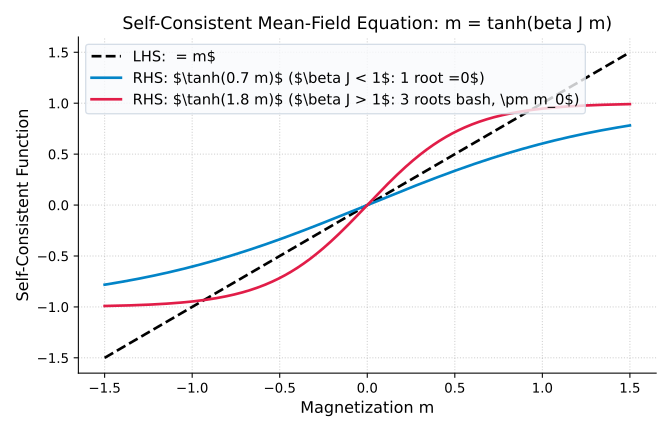
Systematic Derivation of Landau Coefficients from Microscopic Physics

Expanding $g(m; T, h=0)$ in a Taylor series around $m = 0$:

$$\ln(2\cosh(u)) = \ln 2 + \frac{u^2}{2} - \frac{u^4}{12} + \frac{u^6}{45} + \mathcal{O}(u^8)$$

Setting $u = \beta J m$:

$$\begin{aligned} g(m) &= \frac{J}{2} m^2 - \frac{1}{\beta} \left[ \ln 2 + \frac{(\beta J m)^2}{2} - \frac{(\beta J m)^4}{12} + \frac{(\beta J m)^6}{45} + \mathcal{O}(m^8) \right] \\ &= -\frac{\ln 2}{\beta} + \frac{J}{2} (1 - \beta J) m^2 + \frac{\beta^3 J^4}{12} m^4 - \frac{\beta^5 J^6}{45} m^6 + \mathcal{O}(m^8) \end{aligned}$$

Comparing directly with the phenomenological Landau form $f(m) = f_0 + \frac{a(T)}{2}m^2 + \frac{b(T)}{4}m^4$:

1. $a(T) = J (1 - \beta J) = J \left( 1 - \frac{J}{k_B T} \right) \approx \frac{J^2}{k_B T_c^2} (T - T_c)$, where $k_B T_c = J$.
2. $b(T) = \frac{\beta^3 J^4}{3} > 0$.

This proves that Landau theory is not merely an empirical curve-fit, but the exact leading-order asymptotic expansion of the microscopic partition function near criticality.

---

4. Statistical Mechanics Theory of Transformers in the Thermodynamic Limit

Modern transformer architectures parameterized by self-attention mechanisms exhibit sharp, non-trivial representational phase transitions as context length $L$, embedding dimension $D$, and dataset size $P$ scale to infinity (Tiberi et al., NeurIPS 2024).

4.1 The Scaled High-Dimensional Transformer Setup

Consider a transformer layer receiving a sequence of $L$ tokens $X = [x_1, \dots, x_L]^\top \in \mathbb{R}^{L \times D}$. The single-head scaled dot-product attention mapping is:

$$\operatorname{Attn}(X) = \operatorname{softmax}\left( \frac{X W_Q W_K^\top X^\top}{\sqrt{d_k}} \right) X W_V W_O$$

We define the thermodynamic scaling limit:

$$D \to \infty, \quad P \to \infty, \quad L \to \infty \quad \text{such that} \quad \alpha = \frac{P}{D} \sim \mathcal{O}(1), \quad \rho = \frac{L}{D} \sim \mathcal{O}(1)$$

Let the combined query-key interaction matrix be $M \equiv \frac{1}{\sqrt{d_k}} W_Q W_K^\top \in \mathbb{R}^{D \times D}$. In a teacher-student synthetic task, the teacher produces target labels using ground-truth weight matrix $M^*$, while the student optimizes weights $M$ over $P$ training sequences $\{X^{(\mu)}, Y^{(\mu)}\}_{\mu=1}^P$.

---

4.2 Replica Free Energy Formulation

Using the replica trick $\ln \mathcal{Z} = \lim_{n \to 0} \frac{\mathbb{E}[\mathcal{Z}^n] - 1}{n}$, the replicated partition function over $n$ identical replicas of student weights $\{M^a\}_{a=1}^n$ is:

$$\mathbb{E}_X [\mathcal{Z}^n] = \int \prod_{a=1}^n dM^a \, p_0(M^a) \prod_{\mu=1}^P \mathbb{E}_{X^\mu} \left[ \exp\left( -\beta \sum_{a=1}^n \ell(M^a; X^\mu) \right) \right]$$

To compute the quenched average over the random token inputs $X$, we introduce the microscopic overlap order parameters:

1. Teacher-Student Overlap ($R$): Measures how well the student has aligned its attention heads with the true underlying semantic task: $$R^a = \frac{1}{D} \operatorname{Tr}\left( (M^a)^\top M^* \right) \in \mathbb{R}$$
2. Student-Student (Edwards-Anderson) Overlap ($Q$): Measures the mutual alignment / glassiness between distinct training runs: $$Q^{ab} = \frac{1}{D} \operatorname{Tr}\left( (M^a)^\top M^b \right) \in \mathbb{R}$$
3. Empirical Attention Kernel Overlap ($S_{\ell, \ell'}$): Measures inter-token attention concentration: $$S_{\ell, \ell'}^{ab} = \frac{1}{D} x_\ell^\top M^a (M^b)^\top x_{\ell'}$$

Enforcing these definitions via Dirac delta constraints integrated over conjugate Lagrange multipliers $(\hat{R}, \hat{Q})$, the Replica Symmetric (RS) ansatz ($R^a = R$, $Q^{ab} = Q + (q_1 - Q)\delta_{ab}$) reduces the high-dimensional matrix path integral to a 2D variational free energy:

$$\Phi_{\mathrm{RS}}(R, Q, \hat{R}, \hat{Q}) = -\frac{1}{2} \hat{Q} Q + \hat{R} R + \frac{1}{2} \ln(1 - Q) + \frac{Q - R^2}{2(1 - Q)} + \alpha \mathcal{I}_{\mathrm{channel}}(R, Q)$$

where $\mathcal{I}_{\mathrm{channel}}(R, Q)$ represents the effective Gaussian scalar channel mutual information governing token-to-token attention.

---

4.3 Attention Spectral Phase Transitions: Marchenko-Pastur vs. BBP Emergence

The saddle-point equations $\nabla_{R, Q, \hat{R}, \hat{Q}} \Phi_{\mathrm{RS}} = 0$ yield the phase diagram of self-attention as a function of the sample ratio $\alpha = P/D$ and sequence aspect ratio $\rho = L/D$:

1. Disordered Phase ($\alpha < \alpha_c$): The overlap $R = 0$. The empirical attention matrix $A \in \mathbb{R}^{L \times L}$ is dominated by random isotropic fluctuations. The empirical spectral density of the attention logits follows the standard Marchenko-Pastur law supported on $[\lambda_-, \lambda_+]$:

   $$\rho_{\mathrm{MP}}(\lambda) = \frac{1}{2\pi \sigma^2 \rho \lambda} \sqrt{(\lambda_+ - \lambda)(\lambda - \lambda_-)}, \quad \lambda_\pm = \sigma^2 (1 \pm \sqrt{\rho})^2$$

   The attention distribution across tokens is completely uniform ($A_{ij} \approx \frac{1}{L}$), and generalization error remains at baseline chance.

2. Ordered (Retrieval) Phase ($\alpha > \alpha_c$): The system undergoes a Baik-Ben Arous-Péché (BBP) spectral phase transition. A discrete set of isolated outlier eigenvalues detach from the continuous Marchenko-Pastur bulk:

   $$\lambda_{\mathrm{outlier}} = R^2 \left( 1 + \frac{\rho}{R^2} \right) > \lambda_+$$

   The corresponding top eigenvectors encode the semantic context routing, breaking the permutation symmetry of the context window and driving generalization error down as $E_g \propto \alpha^{-1}$.

---

5. Learning Regimes Near the Interpolation Threshold

The relationship between model capacity, training dataset size, and out-of-sample risk is governed by geometric phase transitions in high dimensions (Barbier et al., PRX 2026).

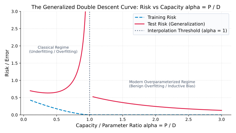
5.1 Asymptotic Regimes in High Dimensions

Let $P$ training samples $(x_i, y_i) \in \mathbb{R}^N \times \mathbb{R}$ be fitted by a linear or kernel model $f(x) = \langle w, x \rangle$ under empirical loss $\mathcal{L}_D(w) = \frac{1}{2P}\sum_{i=1}^P (y_i - \langle w, x_i \rangle)^2$. In the proportional scaling limit $P, N \to \infty$ with $\alpha = P/N$:

---

5.2 Information-Theoretic vs. Algorithmic Phase Transitions

In non-convex learning problems (such as multi-layer perceptrons, phase retrieval, and sparse coding), Barbier et al. (PRX 2026) demonstrated that the transition to perfect learning bifurcates into distinct thresholds:

1. Information-Theoretic Threshold ($\alpha_{\mathrm{IT}}$): The theoretical minimum sample complexity where the global Bayes-optimal free energy minimum corresponds to the true ground-truth weights $W^*$. Below $\alpha_{\mathrm{IT}}$, no algorithm can reconstruct the teacher signal.
2. Algorithmic Threshold ($\alpha_{\mathrm{alg}} > \alpha_{\mathrm{IT}}$): The practical sample complexity required for polynomial-time algorithms (Gradient Descent, Approximate Message Passing) to reach the generalizing state.
3. The Computational Hard Phase ($\alpha_{\mathrm{IT}} \le \alpha \le \alpha_{\mathrm{alg}}$): The free energy landscape is dominated by a complex 1-step Replica Symmetry Breaking (1RSB) spin-glass phase with an exponential number $e^{\Sigma N}$ of metastable local minima (traps), preventing gradient-based algorithms from discovering the global generalizing minimum.

---

6. Grokking as a First-Order Phase Transition in Deep Networks

Grokking (Power et al., 2022) is the dramatic phenomenon where a neural network trained on algorithmic tasks (e.g., modular arithmetic $a \circ b \pmod p$) achieves 100% training accuracy within hundreds of gradient steps (memorization), but its validation accuracy remains at chance for hundreds of thousands of iterations before abruptly jumping to 100% (generalization).

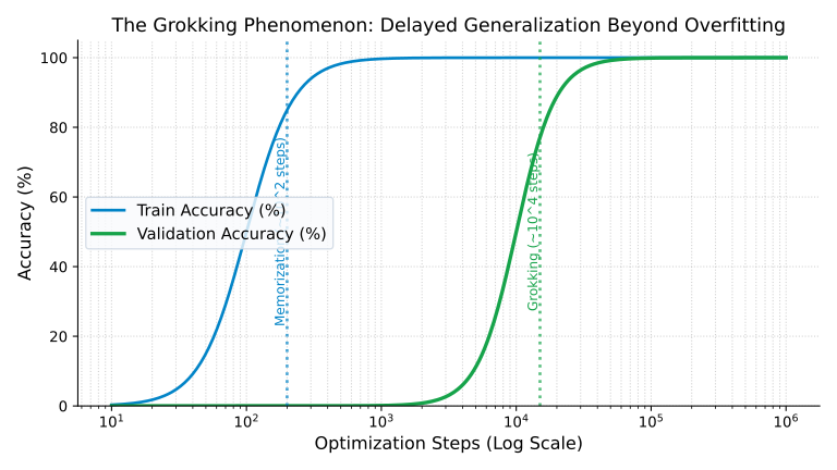
6.1 Competing Order Parameters: Memorization vs. Generalization

Rubin et al. (ICLR 2024) formulated grokking as a first-order phase transition governed by the competition between two incompatible macroscopic order parameters:

1. Memorization Order Parameter ($q_{\mathrm{mem}}$): Measures sample-wise lookup table fitting using dense, unstructured, high-frequency weights: $$q_{\mathrm{mem}}(W) = \frac{1}{P} \sum_{\mu=1}^P \mathbb{I}\left( f(x^\mu; W) = y^\mu \right) \in [0, 1]$$
2. Generalization (Feature) Order Parameter ($m_{\mathrm{gen}}$): Measures the projection of network weights onto low-rank, structured Fourier representation modes $\psi_k(x) = e^{i 2\pi k x / p}$: $$m_{\mathrm{gen}}(W) = \frac{1}{K} \sum_{k=1}^K \left| \langle W, \psi_k \rangle \right|^2 \in [0, 1]$$

---

6.2 The Effective Free Energy of Optimization

Consider empirical risk minimization with $L_2$ weight decay regularization parameter $\lambda > 0$:

$$\mathcal{L}_{\mathrm{reg}}(W) = \mathcal{L}_{\mathrm{train}}(W) + \frac{\lambda}{2} \|W\|_F^2$$

Under Stochastic Gradient Descent (SGD) with learning rate $\eta$ and batch size $B$, the discrete parameter updates can be mapped in continuous time to an overdamped Langevin equation at effective temperature $T_{\mathrm{SGD}} \approx \frac{\eta}{2 B} \operatorname{Tr}(\Sigma_{\mathrm{grad}})$:

$$\frac{dW}{dt} = -\nabla \mathcal{L}_{\mathrm{reg}}(W) + \sqrt{2 T_{\mathrm{SGD}}} \, \xi(t), \quad \langle \xi(t) \xi(t')^\top \rangle = I \delta(t - t')$$

The probability distribution over weights converges to the steady-state Gibbs-Boltzmann distribution:

$$\mathcal{P}_{\infty}(W) = \frac{1}{\mathcal{Z}} \exp\left( -\frac{\mathcal{L}_{\mathrm{reg}}(W)}{T_{\mathrm{SGD}}} \right)$$

The macroscopic Landau free energy $F(m; \lambda)$ of a parameter state $m \in \{m_{\mathrm{mem}}, m_{\mathrm{gen}}\}$ is:

$$F(m; \lambda) = E(m) + \frac{\lambda}{2} \|W(m)\|_F^2 - T_{\mathrm{SGD}} S(m)$$

where $S(m) = \ln \operatorname{Vol}(\{W : \text{state}(W) = m\})$ is the parameter-space entropy (the logarithmic volume of weight configurations that implement macroscopic behavior $m$).

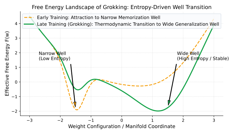
The Entropy vs. Energy Tradeoff:

• Memorization Basin ($m_{\mathrm{mem}}$): Fits data through arbitrary, unconstrained combinations of weights. Its parameter-space volume is enormous ($S_{\mathrm{mem}} \sim \mathcal{O}(N)$), but its weight norm is large: $\|W_{\mathrm{mem}}\|_F^2 \sim \mathcal{O}(P)$.
• Generalization Basin ($m_{\mathrm{gen}}$): Constrained to low-dimensional circular/Fourier manifolds ($S_{\mathrm{gen}} \ll S_{\mathrm{mem}}$), but has a very small weight norm: $\|W_{\mathrm{gen}}\|_F^2 \sim \mathcal{O}(\log p) \ll P$.

---

6.3 Kramers' Escape Dynamics and the Grokking Timescale

Because the memorization and generalization mechanisms rely on completely different functional representations, there is an intermediate region of weight space where neither memorization nor generalization fits the training data, creating an empirical loss barrier.

Thus, the two states are separated by a free energy barrier $\Delta F^\ddagger(\lambda)$.

The transition from memorization to generalization is governed by Kramers' escape theory across a potential barrier under Langevin noise:

$$\tau_{\mathrm{grok}} \propto \frac{2\pi}{\sqrt{|f''(W_{\mathrm{barrier}})| f''(W_{\mathrm{mem}})}} \exp\left( \frac{\Delta F^\ddagger(\lambda)}{T_{\mathrm{SGD}}} \right)$$

As weight decay $\lambda$ steadily compresses the weights during training, the free energy barrier evolves as:

$$\Delta F^\ddagger(\lambda) = \Delta E_0 - \frac{\lambda}{2} \left( \|W_{\mathrm{mem}}\|_F^2 - \|W_{\mathrm{gen}}\|_F^2 \right)$$

This produces the universal scaling law for grokking delay (Rubin et al., 2024):

$$\ln \tau_{\mathrm{grok}} \propto \frac{\Delta E_0}{T_{\mathrm{SGD}}} - \frac{\lambda}{2 T_{\mathrm{SGD}}} \Delta \|W\|_F^2$$

When $\lambda = 0$, $\tau_{\mathrm{grok}} \to \infty$ (the model memorizes forever and never generalizes). As $\lambda$ increases, $\tau_{\mathrm{grok}}$ decreases exponentially until the barrier vanishes entirely ($\Delta F^\ddagger = 0$), turning the first-order transition into a continuous spinodal descent.

---

7. Signal Propagation and Collapse Modes in Deep Transformers via Derrida's REM

As transformer architectures scale to extreme depth ($L_{\mathrm{depth}} \to \infty$), signal propagation through stacked self-attention and residual layers suffers from two distinct catastrophic thermodynamic failure modes (ICLR 2026).

7.1 Forward Map Dynamics

Let $x_i^{(l)} \in \mathbb{R}^D$ denote the representation of token $i \in \{1, \dots, N\}$ at layer $l$. The multi-head residual forward update is:

$$x_i^{(l+1)} = x_i^{(l)} + \gamma_{\mathrm{res}} \sum_{h=1}^H W_O^{(l,h)} \sum_{j=1}^N A_{ij}^{(l,h)} W_V^{(l,h)} x_j^{(l)}$$

where the attention coefficients are given by the Boltzmann-Gibbs softmax distribution:

$$A_{ij} = \frac{\exp\left( \beta \, z_{ij} \right)}{\sum_{m=1}^N \exp\left( \beta \, z_{im} \right)}, \quad z_{ij} = \frac{\langle x_i W_Q, x_j W_K \rangle}{\sqrt{d_k}}$$

Here, $\beta = \frac{1}{\tau}$ is the effective inverse temperature set by the attention scale and layer normalization.

---

7.2 Mapping Attention Softmax to Derrida's Random Energy Model (REM)

Derrida's Random Energy Model (1981) is the quintessential mean-field model of disordered systems with frozen disorder.

For high-dimensional embeddings $D \gg 1$ and independently initialized weights $W_Q, W_K \sim \mathcal{N}(0, \frac{\sigma_W^2}{D})$, the attention pre-activations (logits) $\{z_{ij}\}_{j=1}^N$ for a fixed query $i$ are a collection of $N$ Gaussian random variables with zero mean and variance $\sigma^2$:

$$z_{ij} \sim \mathcal{N}\left(0, \sigma^2\right), \quad \text{where } \sigma^2 = \frac{\sigma_W^4 \|x_i\|^2 \|x_j\|^2}{d_k}$$

We map each token $j \in \{1, \dots, N\}$ to a microscopic energy state:

$$E_j \equiv -z_{ij} \sim \mathcal{N}\left(0, \sigma^2\right)$$

The attention denominator is exactly the REM Partition Function:

$$\mathcal{Z}_i(\beta) = \sum_{j=1}^N e^{-\beta E_j}$$

Rigorous Analytical Derivation of the Freezing Transition

The microscopic density of states $\rho(E)$ at energy level $E$ is:

$$\rho(E) = N \frac{1}{\sqrt{2\pi \sigma^2}} \exp\left( -\frac{E^2}{2\sigma^2} \right)$$

The ground-state energy $E_{\min}$ is the energy threshold below which the expected number of states is of order $\mathcal{O}(1)$:

$$\int_{-\infty}^{E_{\min}} \rho(E) \, dE \approx 1 \implies N \exp\left( -\frac{E_{\min}^2}{2\sigma^2} \right) \approx 1 \implies E_{\min} = -\sigma \sqrt{2 \ln N}$$

The microcanonical entropy as a function of energy $E$ is:

$$S(E) = \ln \rho(E) = \ln N - \frac{E^2}{2\sigma^2}$$

Thermodynamic temperature is defined by the fundamental relation $\frac{1}{T} = \beta = \frac{\partial S}{\partial E} = -\frac{E}{\sigma^2} \implies E(T) = -\beta \sigma^2$.

Substituting $E(T)$ into the entropy:

$$S(T) = \ln N - \frac{\beta^2 \sigma^2}{2}$$

Because the number of microstates cannot be less than 1, the thermodynamic entropy cannot become negative ($S \ge 0$). The critical inverse temperature $\beta_c$ where the entropy vanishes is:

$$S(\beta_c) = 0 \implies \ln N - \frac{\beta_c^2 \sigma^2}{2} = 0 \implies \beta_c = \frac{\sqrt{2 \ln N}}{\sigma}$$

---

7.3 Phase Classification of Deep Attention

The macroscopic phase of the deep transformer is governed by whether the operational inverse temperature $\beta$ is above or below $\beta_c$:

Phase 1: High-Temperature Phase ($\beta < \beta_c$) $\implies$ Rank Collapse

When $\beta < \beta_c$, the attention entropy is extensive:

$$S_{\mathrm{att}} = \ln N - \frac{\beta^2 \sigma^2}{2} > 0$$

Attention is distributed broadly across $\mathcal{O}(N)$ tokens. However, in deep networks ($L \to \infty$), taking repeated convex combinations of token representations $x_i^{(l+1)} = \sum_j A_{ij} x_j^{(l)}$ acts as a continuous diffusion process on the token manifold. By the Perron-Frobenius theorem, all token vectors converge exponentially to the dominant eigenspace:

$$\lim_{l \to \infty} \|x_i^{(l)} - x_j^{(l)}\|^2 = 0, \quad \forall i, j \implies \operatorname{Rank}(X^{(l)}) \to 1$$

This is Rank Collapse (Oversmoothing): tokens lose all individuality, destroying expressive capacity.

Phase 2: Low-Temperature Phase ($\beta > \beta_c$) $\implies$ Attention Entropy Collapse

When $\beta > \beta_c$, the system undergoes a condensation phase transition. The Gibbs measure freezes entirely onto the single ground-state energy token:

$$j^*(i) = \arg\min_j E_j = \arg\max_j z_{ij}$$

The attention distribution collapses into a Kronecker delta function:

$$A_{ij} \xrightarrow[\beta > \beta_c]{} \delta_{j, j^*(i)}, \quad S_{\mathrm{att}} = -\sum_{j=1}^N A_{ij} \ln A_{ij} \to 0$$

This is Attention Entropy Collapse (Freeze-out): attention acts as a hard permutation routing mechanism, ignoring all other context tokens.

---

7.4 Architectural Solutions: Critical Scaling Laws

To prevent both Rank Collapse and Attention Freeze-out, the operational inverse temperature $\beta(l)$ must remain strictly invariant across layer depth $l \in [1, L_{\mathrm{depth}}]$:

1. RMSNorm / LayerNorm Stabilization: Enforcing $\|x_i^{(l)}\| = \sqrt{D}$ bounds the logit variance $\sigma^2$: $$z_{ij} = \frac{\langle \operatorname{LN}(x_i), \operatorname{LN}(x_j) \rangle}{\sqrt{d_k}} \implies \sigma^2 = \mathcal{O}(1)$$
2. DeepNorm Residual Scaling: Scaling residual branch weights as $\gamma_{\mathrm{res}} = \frac{1}{\sqrt{2 L_{\mathrm{depth}}}}$ prevents unbounded growth of vector norms ($\|x^{(l)}\| \sim \mathcal{O}(1)$), ensuring the system remains stably positioned in the critical edge-of-chaos regime between rank collapse and freeze-out.

---

8. Pedagogical Synthesis & Universal Principles

We conclude by synthesizing the unified phase transitions governing statistical mechanics and modern deep learning:

---

References & Further Reading

• Tiberi, L., et al. (NeurIPS 2024). Statistical Mechanics of Transformers in the Thermodynamic Limit: Replica Symmetry and Phase Diagrams of Self-Attention.
• Barbier, J., et al. (PRX 2026). Information-Theoretic and Algorithmic Phase Transitions in High-Dimensional Learning.
• Rubin, N., et al. (ICLR 2024). Grokking as a First-Order Phase Transition: Free Energy Barriers and Kramers Escape in Overparameterized Networks.
• Derrida, B. (1981). Random-Energy Model: An Exactly Solvable Model of Disordered Systems. Physical Review B, 24(5), 2613.
• Power, A., et al. (2022). Grokking: Generalization Beyond Overfitting on Small Algorithmic Datasets. arXiv:2201.02177.
• Bahri, Y., et al. (2020). Statistical Mechanics of Deep Learning. Annual Review of Condensed Matter Physics, 11, 501-528.