Lecture 11.2: Markov Chains and Hidden Markov Models
A comprehensive analysis of Markov Chains, state properties, stationary distributions, and Hidden Markov Models (HMM).
When modelling sequential processes over time (like weather patterns, speech phonemes, or web page navigation paths), variables are rarely independent. A Markov Chain is a statistical model designed to represent sequences of events where transitions from state to state are governed by probability.
The Markov Property (Memorylessness)
A Markov Chain operates under a crucial assumption known as the Markov Property:
The future state in a sequence depends only on the current state. The path taken to reach the current state has no bearing on the future.
Mathematically, a sequence of random states satisfies the Markov property if:
This memoryless assumption significantly reduces computational complexity since we only need to store the current state to predict future steps.
State Transition Matrix
The probabilities of transitioning from any state to another in a single step are organized into a square matrix called the State Transition Matrix ().
For a system with states, is a matrix where element represents the probability of transitioning from state to state :
Key Characteristics:
- Row-Stochastic: Because a state must transition to one of the possible system states, the sum of probabilities in each row must equal exactly one:
Concrete Examples
1. Weather Transition Scenario (2 States: Sunny, Rainy)
Suppose weather transitions are modeled as:
- If it is Sunny today, the probability of it being Sunny tomorrow is , and Rainy is .
- If it is Rainy today, the probability of it being Rainy tomorrow is , and Sunny is .
The corresponding transition matrix is:
| From \ To | Sunny | Rainy |
|---|---|---|
| Sunny | ||
| Rainy |
2. Web Page Navigation Scenario (3 States: Home, About, Contact)
A user browsing a website transitions between pages with probabilities represented by:
Types of States in a Markov Chain
Different configurations of paths in a Markov chain yield various state classifications:
- Transient State: A state that, once left, has a non-zero probability of never being visited again.
- Recurrent State: A state to which the process is guaranteed to return eventually (with probability ).
- Absorbing State: A state that is impossible to leave once entered (transition probability ).
- Periodic State: A state that can only be returned to in multiples of a fixed number of steps (e.g., you can only return to it on steps ).
- Aperiodic State: A state with no fixed return cycles ().
- Ergodic State: A state that is recurrent, aperiodic, and positive recurrent (finite expected return time). If all states in a chain are ergodic, the chain is ergodic.
- Accessible State: State is accessible from state if there is a path of transitions with non-zero probability leading from to .
- Communicating States: States and communicate if they are mutually accessible ( and ).
Hidden Markov Model (HMM)
In a standard Markov Chain, every state is directly observable. However, in many real-world systems, the true physical states are hidden from us, and we can only observe indirect outcomes (emissions) generated by those states.
A Hidden Markov Model (HMM) extends the Markov Chain by separating the hidden states from the observable events.
Components & Topology of an HMM
An HMM is mathematically defined by the tuple :
- Hidden States ( or ): A set of underlying states that transition according to the Markov property.
- Transition Matrix (): An matrix representing probabilities of moving between hidden states.
- Observations (): A set of possible observable events .
- Emission Matrix (): An matrix representing the probability of observing event when in hidden state :
- Initial Distribution (): A vector representing the probability of starting in each hidden state at time .
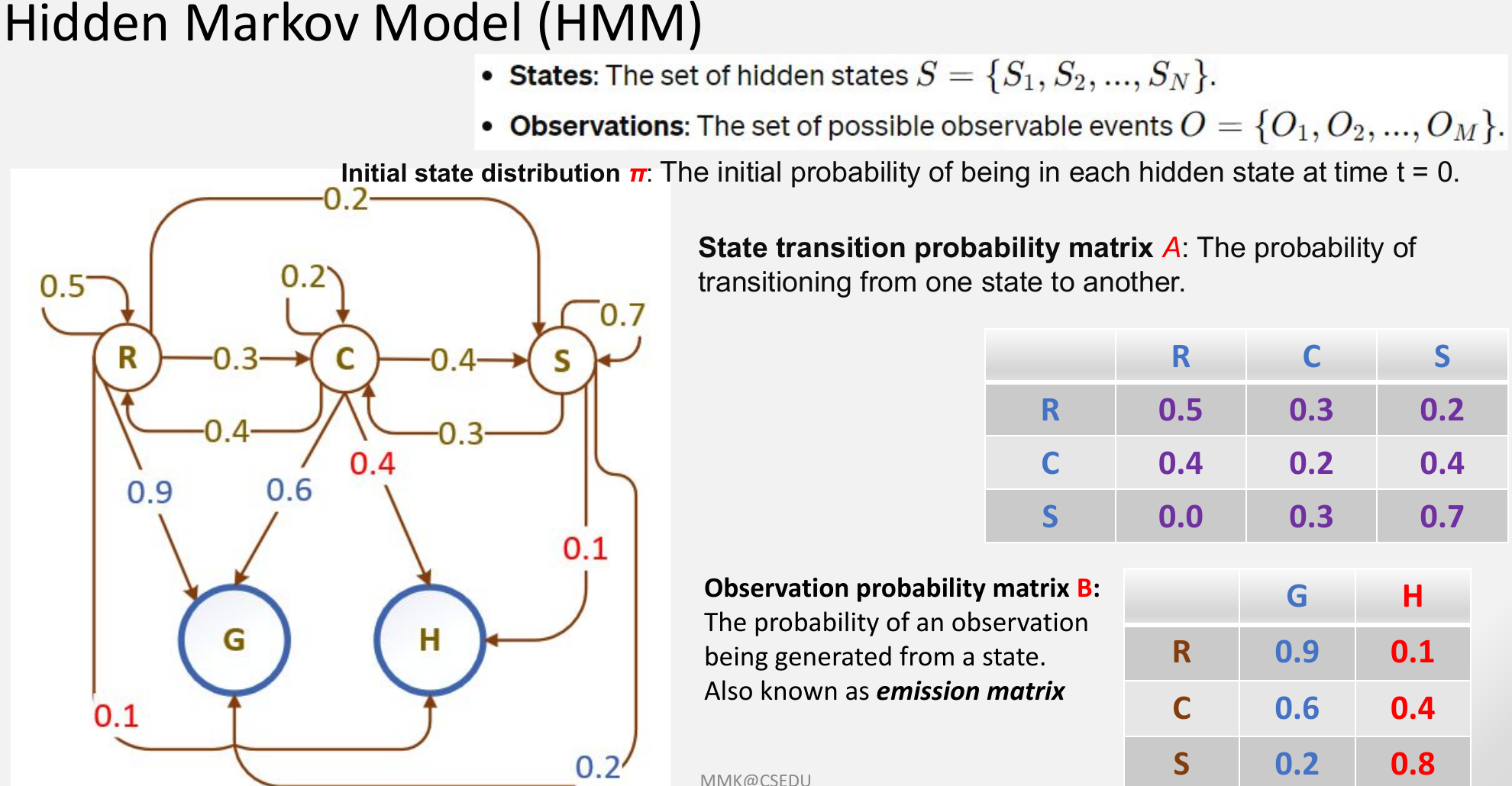
Worked HMM Numerical Trace Example
Using the HMM parameters shown in the slide figure above:
- States ():
- Observations ():
- Initial State Distribution ():
- Transition Matrix ():
- Emission Matrix ():
Step 1: Compute Unobserved Hidden State Distribution at Step
Multiplying by transition matrix :
Step 2: Compute Total Probability of Observing (Go Out)
Summing over all possible hidden states that could emit :
Step 3: Update Posterior Hidden State Probabilities (Bayes Filter Update)
Using Bayes' rule to update the probability of each hidden state given observation :
[!TIP] Interpretation: Observing the agent go out () significantly increases our belief that the weather state is Rainy () or Cloudy (), while dropping the probability of Sunny to because is low.
Classical Example: Eisner's Ice Cream Diary
Suppose we want to reconstruct Baltimore's daily summer weather history (Hidden States: Hot (H) vs. Cold (C)) solely using Jason Eisner's diary entries listing the number of ice creams he ate each day (Observations: 1, 2, or 3 ice creams).
- Weather states (H, C) follow a Markov transition matrix .
- Ice cream counts (1, 2, 3) are emitted from those weather states with probabilities in emission matrix (e.g., eating 3 ice creams is highly likely on a Hot day but rare on a Cold day).
Stationary Distribution
A stationary distribution is a probability distribution over states that remains unchanged after applying the transition matrix. It satisfies the matrix equation:
Where . In an ergodic Markov chain, the system will eventually converge to this unique stationary distribution regardless of the initial starting state.
Step-by-Step Numerical Example
Consider a 3-state Markov chain (States: , , ) with the transition matrix:
Let the current state probability distribution at step be:
To calculate the probability distribution at step , we multiply by the transition matrix :
So the updated distribution is:
If we repeat this multiplication many times, the distribution stabilizes. For this matrix, the stationary distribution converges to:
This means that in the long run, the system will spend approximately of the time in state , in state , and in state .
The Three Fundamental Problems in HMMs
Working with Hidden Markov Models involves solving three core problems:
1. The Evaluation Problem
- Question: Given HMM parameters and an observation sequence , what is the probability that this sequence was generated by the model?
- Solution: Solved efficiently in time using the Forward Algorithm or Backward Algorithm (dynamic programming algorithms that sum probabilities over all possible hidden paths).
2. The Decoding Problem
- Question: Given HMM parameters and an observation sequence , what is the most likely sequence of hidden states that produced the observations?
- Solution: Solved using the Viterbi Algorithm, which utilizes dynamic programming and backtracking to find the single "maximum probability path" (Viterbi path) through the hidden states.
3. The Learning Problem
- Question: Given only an observation sequence and a set of states, how do we learn the optimal HMM parameters that maximize ?
- Solution: Solved using the Baum-Welch Algorithm (a specialized case of the Expectation-Maximization (EM) algorithm) which iteratively estimates state transitions and emissions to converge on local likelihood maxima.
Lecture 11.1: Probabilistic Reasoning and Bayesian Networks
An in-depth guide to Bayesian reasoning, conditional and joint probability updates, law of total probability, and Bayesian Network inference.
Question Pattern & Exam Analysis
Analysis of CS-4101 Artificial Intelligence Exam Patterns (2022–2024)