Lecture 06.2: Minimax and Alpha-Beta Pruning

While single-move games rely on simultaneous choices, many real-world strategic games (like Chess, Go, or Tic-Tac-Toe) are Sequential Games. Players move alternately in turns, with full knowledge of the history of previous choices.

[!NOTE] Sequential Games vs. Simultaneous Equilibrium: In simultaneous games, we evaluate Nash Equilibria over static payoff matrices. However, standard Nash equilibrium in sequential games can allow non-credible off-equilibrium threats. Minimax (via backward induction) resolves this by enforcing optimal play at every subtree.

Optimal Decisions: The Minimax Algorithm

In a two-player, zero-sum game, we define the players as MAX and MIN.

• MAX prefers to move to a state of maximum utility value.
• MIN prefers to move to a state of minimum utility value.

The Minimax Value of a node is the utility of being in that state, assuming that both players play optimally from that node to the end of the game.

$\text{Minimax}(s) = \begin{cases} \text{Utility}(s) & \text{if } s \text{ is terminal} \\ \max_{a \in \text{Actions}(s)} \text{Minimax}(\text{Result}(s, a)) & \text{if Player}(s) = \text{MAX} \\ \min_{a \in \text{Actions}(s)} \text{Minimax}(\text{Result}(s, a)) & \text{if Player}(s) = \text{MIN} \end{cases}$

Visualizing Minimax State Expansion

Below is a simplified game tree. MAX moves first, followed by MIN.

1. At the bottom, we evaluate the terminal utility values.
2. The MIN nodes (B, C, D) choose the smallest value from their children:
   • $B$ chooses $\min(3, 12, 8) = 3$.
   • $C$ chooses $\min(2, 4, 6) = 2$.
   • $D$ chooses $\min(14, 5, 2) = 2$.
3. The root MAX node ($A$) chooses the largest value from its children:
   • $A$ chooses $\max(3, 2, 2) = 3$.

Thus, MAX's optimal first move is to move to node $B$.

---

Alpha-Beta Pruning

The primary limitation of pure Minimax is that the number of game states it must examine grows exponentially with the tree depth: $O(b^m)$, where $b$ is the branching factor and $m$ is the maximum depth.

Alpha-Beta Pruning computes the exact same optimal minimax decision without examining every node in the game tree. It prunes branches that are guaranteed not to influence the final decision.

Key Parameters

• $\alpha$ (Alpha): The value of the best (highest) choice found so far along the path for MAX. (Initialized to $-\infty$).
• $\beta$ (Beta): The value of the best (lowest) choice found so far along the path for MIN. (Initialized to $+\infty$).

[!IMPORTANT] The Pruning Criterion: Stop exploring a child branch as soon as $\alpha \ge \beta$.

Visualizing Alpha-Beta Pruning

1. The algorithm explores node $B$'s children and determines $B$'s value is $3$.
2. It returns to root $A$. $A$ can guarantee a score of at least $3$, updating $\alpha = 3$.
3. The algorithm moves to node $C$ and evaluates its first child, finding value $2$.
4. Because $C$ is a MIN node, $C$'s value will be $\le 2$.
5. Since root $A$ already has $\alpha = 3$, $A$ will never choose path $C$ (because $3 > 2$).
6. Pruning: The algorithm immediately stops exploring $C$'s remaining children ($4$ and $6$) because $\alpha (3) \ge \beta (2)$.

Complete 6-Stage Alpha-Beta Pruning Walkthrough

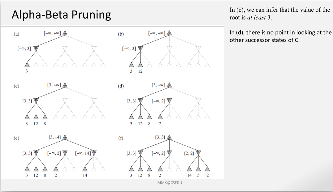
Stage-by-Stage Breakdown:

• Stage (a): Search begins at root $A$ with $\alpha = -\infty, \beta = +\infty$. Moving down to MIN node $B$, we evaluate its first leaf with utility $3$. Node $B$ updates its upper bound to $\beta = 3$, giving bounds $[-\infty, 3]$.
• Stage (b): Node $B$ evaluates its second leaf with utility $12$. Since $\min(3, 12) = 3$, $B$'s upper bound remains $\beta = 3$.
• Stage (c): Node $B$ evaluates its third leaf ($8$). $B$'s final minimax value is $\min(3, 12, 8) = 3$. The algorithm returns to root $A$. Since $A$ is a MAX node, $A$ updates $\alpha = \max(-\infty, 3) = 3$, setting $A$'s bounds to $[3, +\infty]$.

  Key Inference: In stage (c), we can infer that the value of the root $A$ is at least 3.

• Stage (d): Search moves to MIN node $C$ inheriting bounds $[3, +\infty]$. $C$ evaluates its first leaf with utility $2$, updating $C$'s upper bound to $\beta = \min(+\infty, 2) = 2$ (bounds $[-\infty, 2]$).

  Pruning Triggered: Root $A$ already guarantees a payoff of at least $3$ ($\alpha = 3$), while node $C$ guarantees a payoff of at most $2$ ($\beta = 2$). Since $\alpha (3) \ge \beta (2)$, there is no point in looking at the other successor states of $C$. The remaining branches of $C$ are pruned!

• Stage (e): Search moves to MIN node $D$ with inherited bounds $[3, +\infty]$. $D$ evaluates its first leaf ($14$), setting its upper bound to $\beta = 14$ ($[-\infty, 14]$). Root $A$ updates bounds to $[3, 14]$.
• Stage (f): Node $D$ evaluates its remaining leaves ($5$ and $2$), computing $\min(14, 5, 2) = 2$. Node $D$'s value returns $2$ to root $A$. Root $A$ computes $\max(3, 2) = 3$. The final minimax value for root $A$ is 3 (choosing path $B$).

---

Step-by-Step Slide Execution Trace

Below is another step-by-step trace showing $\alpha$ and $\beta$ updates and branch pruning from the lecture slides:

Step 1: Initializing $\alpha, \beta$ and Evaluating $N_4$

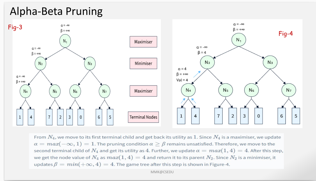
Step 2: Pruning at $N_5$ ($\alpha \ge \beta$)

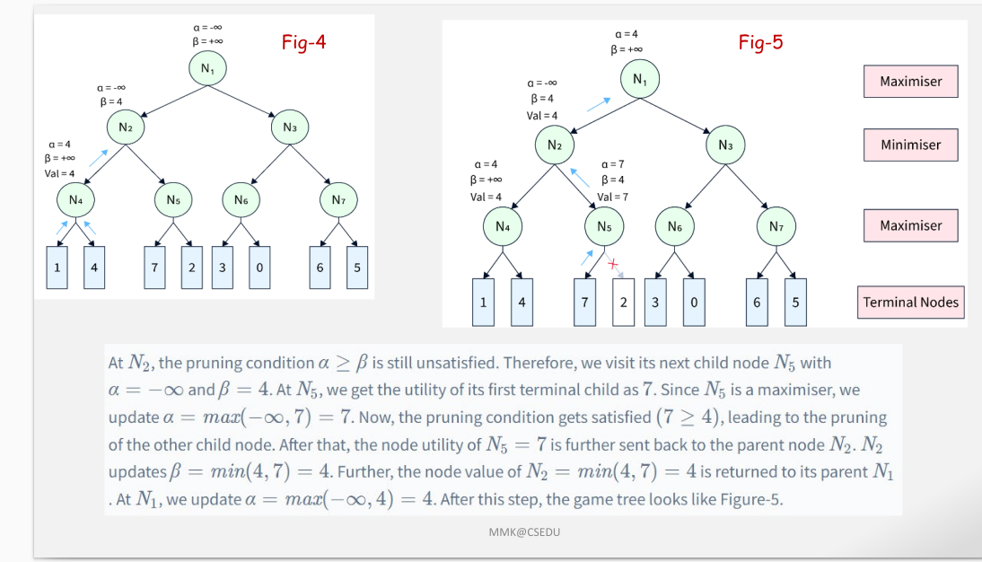
Step 3: Evaluation at $N_6$ and Pruning $N_7$ Subtree

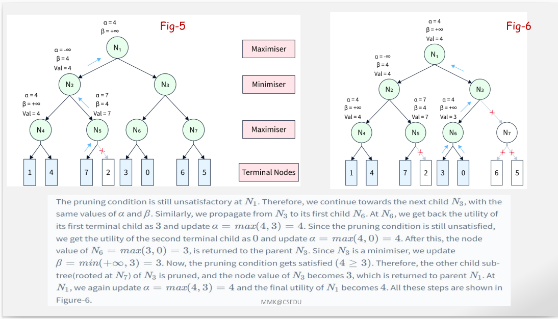
With perfect move ordering, Alpha-Beta pruning reduces time complexity to $O(b^{m/2})$, effectively doubling the searchable depth in the same time frame.

---

Multiplayer Games & Alliances

While two-player zero-sum games utilize a single scalar Minimax value, multiplayer games ($n > 2$ players) evaluate states using utility vectors $\vec{v} = (v_1, v_2, \dots, v_n)$, where component $v_i$ represents the payoff for player $i$.

Alliances in Multiplayer Search

Multiplayer strategic games (such as Risk, Catan, or 3-player Chess) fundamentally introduce alliances—both formal and informal agreements between competing agents:

• Dynamic Alliance Formation: Alliances are made, maintained, and broken dynamically as the game state evolves over time.
• The Counter-Dominance Principle:
  • Suppose players $A$ and $B$ are in relatively weak positions, while player $C$ is in a dominant, leading position.
  • It is optimal for both $A$ and $B$ to form an alliance to jointly attack player $C$ rather than fighting each other, preventing $C$ from destroying each of them individually.
• Dissolution and Betrayal:
  • As soon as player $C$ is sufficiently weakened under joint attacks, the alliance loses its value.
  • At that threshold, either $A$ or $B$ will violate the agreement and attack the former ally to claim sole victory.

[!WARNING] Evaluation Vectors in Multiplayer Games: In multiplayer Minimax ($MAX^n$ algorithm), each player at turn node $i$ chooses the move that maximizes their own component $v_i$ in the payoff vector. Unlike 2-player zero-sum games, explicit collusion or betrayal strategies must be modeled to prevent sub-optimal play.