Lecture 07.1: Constraint Satisfaction Problems and Consistency

In artificial intelligence, problem-solving strategies generally fall into two broad paradigms based on what the search procedure is seeking:

The Constraint Processing Framework

Constraint Processing (pioneered by Rina Dechter) is a general computational framework for modeling and solving problems defined by a set of variables, allowable domain values, and constraints. Constraint processing separates problem modeling into two paradigms:

1. Constraint Satisfaction Problems (CSPs): The objective is simply to find one (or all) assignments of values to variables that satisfy every hard constraint.
2. Constraint Optimization Problems (COPs): The objective goes beyond satisfying hard constraints to optimize a given objective function $f(x)$ (e.g., minimizing cost, execution time, or maximizing resource efficiency) while adhering to constraints.

Formal Definition of a CSP

A Constraint Satisfaction Problem consists of three core components $\langle X, D, C \rangle$:

1. Variables ($X$): A finite set of variables $X = \{X_1, X_2, \dots, X_n\}$.
2. Domains ($D$): A set of domains $D = \{D_1, D_2, \dots, D_n\}$, where each domain $D_i = \{v_1, v_2, \dots, v_k\}$ defines the set of allowable values for variable $X_i$.
3. Constraints ($C$): A set of constraints $\{C_1, C_2, \dots, C_m\}$ specifying allowable combinations of values for subsets of variables.

State & Assignment Terminology

• Partial Assignment: An assignment that attributes values to only a subset of variables in $X$.
• Complete Assignment: An assignment in which every variable $X_i \in X$ has been assigned a value from its domain $D_i$.
• Consistent (Legal) Assignment: An assignment (partial or complete) that does not violate any constraint in $C$.
• Solution: A complete and consistent assignment.

[!NOTE] Why Formalize Problems as CSPs? Standard state-space search requires problem-specific heuristics (e.g., Manhattan distance for 8-puzzle). CSP solvers use a standardized representation pattern, enabling generic goal/successor functions and general-purpose heuristics (such as MRV or Arc Consistency) that operate without domain-specific engineering. Moreover, CSP solvers can rapidly prune massive subtrees of search space.

Varieties of CSP Formalisms

CSPs are categorized based on the nature of their variable domains:

1. Discrete Domains

• Finite Domains: Variables take values from finite sets. For $n$ variables with maximum domain size $d$, the total number of complete assignments is $O(d^n)$.
  • Example: In the 8-Queens Problem, variables $Q_1, \dots, Q_8$ represent queen row positions in columns $1 \dots 8$, with domains $D_i = \{1, 2, 3, 4, 5, 6, 7, 8\}$.
• Infinite Domains: Variables range over infinite discrete sets (e.g., integers $\mathbb{Z}$ or strings).
  • Example: Job shop scheduling without fixed upper deadlines allows start times to grow arbitrarily.
  • Constraint Languages: Since allowable value pairs cannot be explicitly enumerated for infinite domains, a constraint language (e.g., $T_1 + d_1 \le T_2$) must be used directly.

2. Continuous Domains

Common in operations research and real-world engineering:

• Example: Precise scheduling of the Hubble Space Telescope, where continuous variables represent observation start times and pointing angles subject to astronomical, precedence, and power constraints.
• Linear Programming (LP): Continuous CSPs defined by linear equalities and inequalities, solvable in polynomial time relative to variable count.
• Nonlinear Programming: Extensions include Quadratic Programming (QP) and Second-Order Conic Programming (SOCP).

Varieties of Constraints

Constraints can be classified by their scope (number of variables involved) and strictness:

1. Unary Constraints: Restrict the domain of a single variable.
   • Example: $SA \neq \text{green}$.
2. Binary Constraints: Relate pairs of variables.
   • Implicit representation: $SA \neq WA$.
   • Explicit tuple representation: $(WA, NT) \in \{(\text{red}, \text{green}), (\text{red}, \text{blue}), (\text{green}, \text{red}), (\text{green}, \text{blue}), (\text{blue}, \text{red}), (\text{blue}, \text{green})\}$.
3. Higher-Order Constraints: Involve 3 or more variables (e.g., column addition constraints in Crypt-arithmetic puzzles).
4. Global Constraints: Involve an arbitrary number of variables.
   • Note on terminology: The term "global" is traditional but can be misleading; it does not require involving all variables in a problem, but rather an arbitrary list (e.g., Alldiff(X_1, X_2, \dots, X_k) in Sudoku rows/columns).
5. Preference (Soft) Constraints: Specify desirable assignments rated by costs or penalties rather than strict hard limits.
   • Example (Class Assignment): Professor Jan prefers morning slots while Alex prefers afternoon slots. Assigning an afternoon slot to Jan incurs a penalty cost of 2 points, whereas a morning slot costs 1 point.
   • Example (Timetabling): Classroom capacity vs. enrollment is a hard constraint; avoiding simultaneous scheduling of related classes is a soft constraint.

Constraint Graphs

A binary CSP can be represented visually as a Constraint Graph, where nodes represent variables and edges (arcs) represent binary constraints between them.

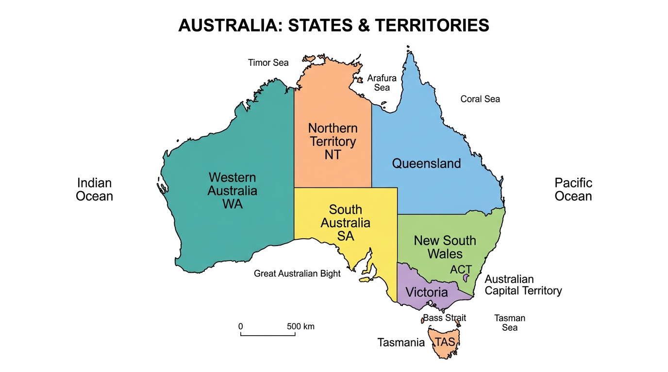
[!TIP] Subproblem Decomposition: Notice that T (Tasmania) is completely disconnected from the rest of the Australian mainland graph. Tasmania is an independent subproblem, which can be solved separately without impacting mainland variable assignments!

Constraint Propagation & Search Space Pruning

Constraint Propagation uses constraints to recursively enforce consistency across variables, shrinking variable domains either as a preprocessing step before search or interleaved during search.

Preprocessing Outcomes

When run as a preprocessing step, constraint propagation produces one of three outcomes:

1. Solves the CSP completely: Reduces every variable domain to size 1 (no search required!).
2. Detects Unsatisfiability: Reduces at least one domain to size 0 (Domain Wipeout / DWO), proving no solution exists.
3. Reduces Search Space: Shrinks domains to smaller sets, simplifying subsequent search.

Quantifying Search Space Reduction

Consider the Australia Map Coloring problem with 7 variables and 3 colors $\{ \text{red}, \text{green}, \text{blue} \}$. Suppose we assign $SA = \text{blue}$.

• Without Constraint Propagation: For the 5 unassigned neighboring variables ($WA, NT, Q, NSW, V$), a naive search procedure must consider: $3^5 = 243 \text{ combinations}$
• With Constraint Propagation: Because $SA = \text{blue}$, the color $\text{blue}$ is immediately removed from the domains of all 5 neighbors. Each neighbor now has only 2 valid options left ($\{ \text{red}, \text{green} \}$): $2^5 = 32 \text{ combinations}$
• Search Space Reduction: $\frac{243 - 32}{243} \approx \mathbf{87\% \text{ reduction}}$ in search states evaluated!

Bounds Consistency

For continuous domains or large integer bounds where enumerating individual domain values is prohibitive, solvers enforce Bounds Consistency.

Instead of tracking discrete sets, domains are represented by continuous or integer intervals $[D_i^{\text{min}}, D_i^{\text{max}}]$. Bounds consistency ensures that for each boundary value of a variable's domain, there exist matching boundary values in adjacent variables that satisfy the constraints.

Example: Airline Transportation Scheduling

Consider scheduling passengers across two airline flights $F_1$ and $F_2$:

• Flight capacities: Flight $F_1$ holds up to 165 passengers; Flight $F_2$ holds up to 385 passengers. $D_1 = [0, 165], \quad D_2 = [0, 385]$
• Constraint: Combined, both flights must carry exactly 420 passengers ($F_1 + F_2 = 420$).

Enforcing Bounds Consistency:

1. To satisfy $F_1 = 420 - F_2$:
   • Minimum possible $F_1 = 420 - \max(F_2) = 420 - 385 = \mathbf{35}$
   • Maximum possible $F_1 = 420 - \min(F_2) = 420 - 0 = 420 \implies \text{capped at capacity } \mathbf{165}$
2. To satisfy $F_2 = 420 - F_1$:
   • Minimum possible $F_2 = 420 - \max(F_1) = 420 - 165 = \mathbf{255}$
   • Maximum possible $F_2 = 420 - \min(F_1) = 420 - 0 = 420 \implies \text{capped at capacity } \mathbf{385}$

The pruned interval domains become: $D_1 = [35, 165], \quad D_2 = [255, 385]$

Hierarchy of Local Consistency

Local consistency algorithms enforce constraint rules on localized subgraphs, propagating removals throughout the network.

1. Node Consistency

A variable $X$ is node-consistent if every value in its domain $D_X$ satisfies all unary constraints $C(X)$ on $X$.

• Formal condition: $\forall v \in D_X, \text{ satisfies } C(v)$.
• Example: Variable $A$ has domain $D_A = \{1, 2, 3, 4\}$ with unary constraint $A > 2$. Pruning values $\{1, 2\}$ leaves $D_A = \{3, 4\}$.

2. Arc Consistency

A variable $X$ is arc-consistent with respect to another variable $Y$ (written as directed arc $X \rightarrow Y$) if for every value $x \in D_X$, there exists at least one value $y \in D_Y$ such that the binary constraint $C(X, Y)$ is satisfied.

• Formal condition: $\forall x \in D_X, \exists y \in D_Y \text{ s.t. } (x, y) \in C_{XY}$.
• If any $x \in D_X$ lacks such supporting $y$, $x$ is removed from $D_X$.

[!IMPORTANT] Arc Consistency is Directed: Arc $X \rightarrow Y$ consistency does not imply $Y \rightarrow X$ consistency. Both directions must be checked and enforced independently.

Concrete Example

• Variables: $X \in \{1, 2, 3\}$, $Y \in \{2, 3\}$
• Constraint: $X < Y$

Check directed arc $X \rightarrow Y$:

1. $X = 1$: Supported by $y = 2$ and $y = 3$ ($1 < 2, 1 < 3$). (Kept)
2. $X = 2$: Supported by $y = 3$ ($2 < 3$). (Kept)
3. $X = 3$: No $y \in D_Y$ satisfies $3 < y$. (Pruned!)

Revised Domain: $D_X = \{1, 2\}$.

3. Path Consistency & K-Consistency

• Path Consistency: Evaluates triples of variables $\{X_i, X_j, X_k\}$. A pair of values $\{x_i, x_j\}$ consistent with binary constraint $C(X_i, X_j)$ is path-consistent with $X_k$ if there exists a value $x_k \in D_k$ satisfying $C(X_i, X_k)$ and $C(X_j, X_k)$.
• K-Consistency: Generalizes local consistency. A CSP is $k$-consistent if for any consistent assignment to $(k-1)$ variables, any $k$-th variable can be assigned a consistent value.
  • 1-consistency = Node consistency.
  • 2-consistency = Arc consistency.
  • 3-consistency = Path consistency.
  • A CSP is strongly $k$-consistent if it is $k$-consistent, $(k-1)$-consistent, ..., down to 1-consistent. If a graph with $n$ variables is strongly $n$-consistent, a solution can be found in $O(n \cdot d)$ time with zero backtracking!

The AC-3 Algorithm

The AC-3 algorithm (Mackworth, 1977) maintains a queue of directed arcs requiring verification. When a domain $D_i$ is pruned, all incoming arcs $(X_k \rightarrow X_i)$ from neighboring variables must be re-queued, because values in $D_k$ that relied on the pruned value for support may now be invalid.

Pseudocode

function AC-3(csp) returns false if inconsistency is found, true otherwise
    inputs: csp, a binary CSP with variables X, domains D, constraints C
    local variables: queue, a queue of arcs, initially containing all arcs in csp
    
    while queue is not empty do
        (Xi, Xj) = REMOVE-FIRST(queue)
        if REVISE(csp, Xi, Xj) then
            if size of Di == 0 then 
                return false // Domain Wipe Out (DWO) - no solution exists
            for each Xk in Xi.NEIGHBORS - {Xj} do
                add (Xk, Xi) to queue
    return true

function REVISE(csp, Xi, Xj) returns true iff we revise the domain of Xi
    revised = false
    for each x in Di do
        if no value y in Dj satisfies the constraint between Xi and Xj then
            delete x from Di
            revised = true
    return revised

Trace Walkthrough: Divisibility Constraint Network

Trace AC-3 on three variables $\{x, y, z\}$ with divisibility constraints:

• Constraints: $z$ divides $x$ and $z$ divides $y$ (i.e., $x/z \in \mathbb{Z}$ and $y/z \in \mathbb{Z}$).
• Initial Domains: $D_x = \{2, 5\}$, $D_y = \{2, 4\}$, $D_z = \{2, 5\}$.

Initial Queue: $\text{Queue} = \{(x, z), (z, x), (y, z), (z, y)\}$

1. Pop $(z, y)$: Check if each $z \in D_z$ divides some $y \in D_y = \{2, 4\}$.
   • $z = 2$: divides $y=2$ and $y=4$. (Kept)
   • $z = 5$: does not divide $2$ or $4$. (Pruned!)
   • Domain update: $D_z = \{2\}$. Re-queue neighbors pointing to $z$: $(x, z)$ is already in queue.
2. Pop $(x, z)$: Check if each $x \in D_x = \{2, 5\}$ has a divisor $z \in D_z = \{2\}$.
   • $x = 2$: divisible by $z=2$. (Kept)
   • $x = 5$: not divisible by $z=2$. (Pruned!)
   • Domain update: $D_x = \{2\}$.
3. Pop $(z, x)$: Check $z \in \{2\}$ divides $x \in \{2\}$. Valid. (No change).
4. Pop $(y, z)$: Check $y \in \{2, 4\}$ is divisible by $z \in \{2\}$. Valid. (No change).

Final Arc-Consistent Domains: $D_x = \{2\}, \quad D_y = \{2, 4\}, \quad D_z = \{2\}$

Comparison of Arc Consistency Algorithms (AC-1 to AC-4)

(Where $n = |X|$ is variable count, $d = \max |D_i|$ is maximum domain size, and $e = |C|$ is binary constraint arc count.)