Lecture 04.2: A* Search and Extensions

Greedy Best-First Search is fast but not optimal, because it only looks at the estimated distance to the goal ($h(n)$) and ignores the cost of the path accumulated so far ($g(n)$).

To achieve optimal search, we want to minimize the overall length of the path. We introduce $g(n)$ as the exact cost of the best path found so far from the initial node to node $n$.

---

A* Search

A Search* combines uniform-cost search (which minimizes path cost $g(n)$) with greedy best-first search (which minimizes estimated goal distance $h(n)$). The core intuition is to avoid expanding paths that are already expensive.

The evaluation function for A* is: $f(n) = g(n) + h(n)$

• $g(n)$: Exact cost so far to reach node $n$ from the initial state.
• $h(n)$: Estimated cost from node $n$ to the nearest goal state.
• $f(n)$: Estimated total cost of the cheapest solution path through node $n$ to a goal.

---

Admissible Heuristics

For A* search to guarantee an optimal solution, the heuristic function $h(n)$ must be admissible.

Let $h^*(n)$ be the true cost of the optimal path from node $n$ to a goal node. A heuristic $h(n)$ is admissible if it never overestimates the cost to reach the goal: $0 \le h(n) \le h^*(n)$

An admissible heuristic is always optimistic. Because an admissible heuristic never overestimates the remaining distance, A* will never mistakenly rule out or skip over a path that could lead to an optimal goal state.

---

Visualizing Step-by-Step A* Expansion

Let's return to finding a route from Arad to Bucharest using $f(n) = g(n) + h(n)$ with $h_{SLD}(n)$:

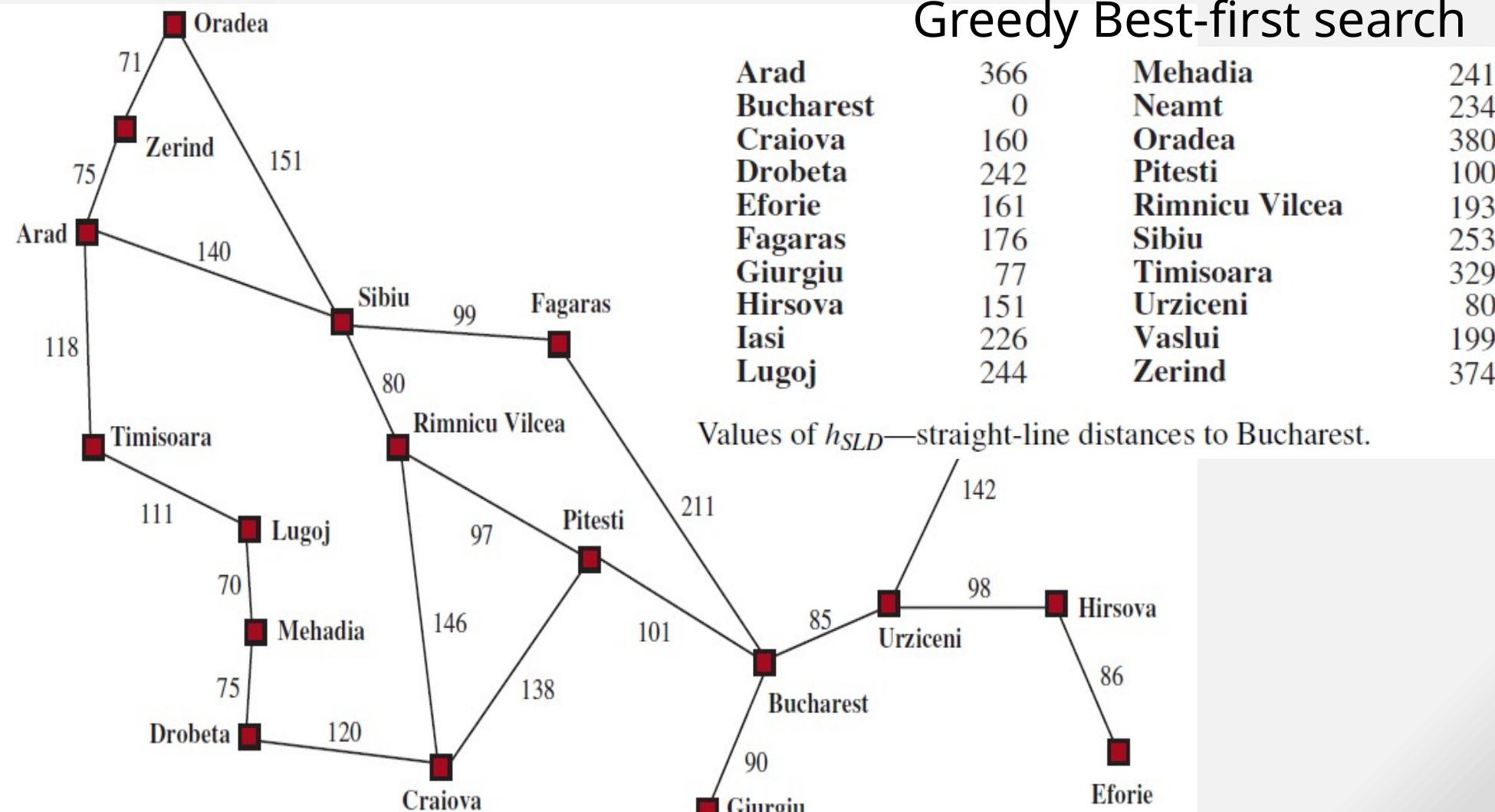
Step-by-Step Search Trace

1. Start at Arad: $g(\text{Arad}) = 0$, $h(\text{Arad}) = 366 \implies f(\text{Arad}) = 366$.
2. Expand Arad:
   • Sibiu: $g = 140, h = 253 \implies f = 393$
   • Timisoara: $g = 118, h = 329 \implies f = 447$
   • Zerind: $g = 75, h = 374 \implies f = 449$
   • Frontier: [Sibiu (393), Timisoara (447), Zerind (449)] $\rightarrow$ Expand Sibiu ($f=393$).
3. Expand Sibiu:
   • Rimnicu Vilcea: $g = 220, h = 193 \implies f = 413$
   • Fagaras: $g = 239, h = 176 \implies f = 415$
   • Arad: $g = 280, h = 366 \implies f = 646$
   • Oradea: $g = 291, h = 380 \implies f = 671$
   • Frontier: [Rimnicu Vilcea (413), Fagaras (415), Timisoara (447), Zerind (449), Arad (646), Oradea (671)] $\rightarrow$ Expand Rimnicu Vilcea ($f=413$).
4. Expand Rimnicu Vilcea:
   • Pitesti: $g = 317, h = 100 \implies f = 417$
   • Craiova: $g = 366, h = 160 \implies f = 526$
   • Sibiu: $g = 300, h = 253 \implies f = 553$
   • Frontier: [Fagaras (415), Pitesti (417), Timisoara (447), Zerind (449), Craiova (526), Sibiu (553)] $\rightarrow$ Expand Fagaras ($f=415$).
5. Expand Fagaras:
   • Bucharest: $g = 450, h = 0 \implies f = 450$
   • Frontier: [Pitesti (417), Timisoara (447), Zerind (449), Bucharest via Fagaras (450), Craiova (526)] $\rightarrow$ A* does not stop yet! Pitesti ($f=417$) has a lower $f$-value than Bucharest via Fagaras ($f=450$). Expand Pitesti ($f=417$).
6. Expand Pitesti:
   • Bucharest: $g = 418, h = 0 \implies f = 418$
   • Frontier: [Bucharest via Pitesti (418), Timisoara (447), Zerind (449), Bucharest via Fagaras (450)] $\rightarrow$ Pop Bucharest via Pitesti ($f=418$). Goal selected from queue!

By evaluating total path cost $f(n) = g(n) + h(n)$, A correctly pivots away from the non-optimal route via Fagaras and finds the optimal path:* $\text{Arad} \rightarrow \text{Sibiu} \rightarrow \text{Rimnicu Vilcea} \rightarrow \text{Pitesti} \rightarrow \text{Bucharest} \quad (\text{Cost} = 418)$

---

Comparison: Greedy Best-First Search vs. A* Search

---

The Effect of the Heuristic Function

The choice of evaluation function drastically alters search behavior:

• Dijkstra’s Algorithm (Uniform-Cost Search): Expands states in order of $f(n) = g(n)$ (equivalent to A* with $h(n) = 0$). It explores outward in all directions equally like ripples in water.
• A Search:* Expands states in order of $f(n) = g(n) + h(n)$. It directs exploration toward the goal, eliminating unnecessary state expansions.
• Weighted A Search:* Expands states in order of $f(n) = g(n) + W \cdot h(n)$, where $W > 1$. This heavily weights estimated remaining distance, speeding up computation while bounding suboptimality to at most $W \times \text{optimal cost}$.

Even with a good heuristic, A* must keep all generated nodes in memory ($O(b^d)$ space complexity) to reconstruct the optimal path and prevent revisit loops, which can lead to memory exhaustion on very large search spaces.

---

Advanced Extensions of A*

To overcome memory limitations and speed up search, several variations of A* exist:

1. Bidirectional A*

• Idea: Runs two simultaneous A* searches—one forward from the start state and one backward from the goal state—meeting in the middle.
• Use Case: Drastically reduces the search tree depth, provided an effective heuristic exists in both directions.

2. Iterative Deepening A* (IDA*)

• Idea: Combines A* evaluation with iterative deepening depth-first search. Instead of limiting depth, each iteration uses an increasing $f$-cost limit (threshold).
• Use Case: Reduces space complexity from exponential $O(b^d)$ to linear $O(bd)$ (like DFS) while retaining A*'s optimality.

3. Beam A*

• Idea: Combines A* with beam search by truncating the frontier to a fixed maximum "beam width" $k$. Only the $k$ best nodes are retained at each level.
• Use Case: Essential when memory is strictly constrained or when an approximate fast solution is acceptable.